Plot an object of class "prova_eu" (expected utility) and its revisability

This base::plot() method is a utility to plot the expected utilities obtained with exputility(), as well as their revisabilities.

Usage

# S3 method for class 'prova_eu'
plot(
  x,
  type = "b",
  lty = c(1, 2, 4, 3, 6, 5),
  pch = c(1, 2, 0, 5, 6, 3),
  lwd = 2,
  col = palette(),
  xlab = NULL,
  ylab = NULL,
  xlim = NULL,
  ylim = NULL,
  legend = "topright",
  add = FALSE,
  alpha.f = 1,
  grid = TRUE,
  lwd.grid = NULL,
  col.grid = "#00000022",
  axes = FALSE,
  main = NULL,
  type.spread = "b",
  lty.spread = 1,
  lwd.spread = 1,
  alpha.f.spread = NULL,
  nsamples.spread = 360,
  ...
)

Arguments

x: Object of class "prova_eu" (expected utility), obtained with exputility().
type: Character vector (default 'b') or list indicating the type of plot for the main probability distribution; see base::plot().
lty: Analogous to argument lty (line style) in graphics::matplot(), used for the main probability distributions.
pch, col, xlab, ylab, main, xlim, ylim, grid, axes, add, lwd.grid, col.grid: see analogous arguments in graphics::plot.default() and graphics::matplot().
lwd: Analogous to argument lwd (line width) in graphics::matplot(), used for the main probability distributions.
legend: One of the values 'bottomright', 'bottom', 'bottomleft', 'left', 'topleft', 'top', 'topright', 'right', 'center' (see graphics::legend()): plot a legend at that position. A value FALSE or any other does not plot any legend. Default 'topright'.
alpha.f: Numeric, default 1: opacity of the colours of lines or markers, 0 being completely invisible and 1 completely opaque.
type.spread: character vector (default 'b') or list indicating the type of plot for the revisability samples; see argument type.
lty.spread: Same as parameter lty (line style), but for the line type of the revisability samples.
lwd.spread: Same as parameter lwd (line width), but for the line type of the revisability samples.
alpha.f.spread: Numeric or NULL (default): opacity of the quantile bands or of the long-run-frequency samples, similar to alpha.f. NULL determines a value dependent on the number of samples (more samples, less opacity).
nsamples.spread: Integer, default 360: number of samples of long-run frequencies to display.
...: Other parameters to be passed to pplot().

Value

NULL, invisibly; produces a plot, see graphics::matplot().

Details

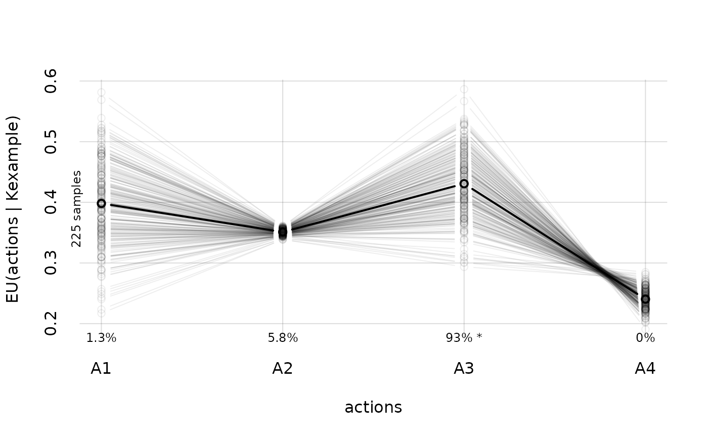
The x-axis spans the possible actions, and the y-axis their expected utilities. Their revisabilities are shown as an ensemble of 360 (default number) expected-utility curves; the number of samples in the ensemble is indicated beside the left y-axis. If any conditioning variate \(X\) was used for the probabilities, \(\mathrm{Pr}(\dotso \vert X = x, \dotso)\), then one such plot is displayed for each conditioning value \(x\).

The probability that an action would still be considered optimal, if many moro learning data were collected, is indicated above the x-axis label corresponding to that action. An asterisk * marks the optimal actions. If any conditioning variate \(X\) was used, then one such probability is shown for each conditioning value.

Examples

## Use the example "prova_K" (knowledge) object 'Kexample'
## calculated from the "penguins" dataset;
## variates: 'species' and 'bill_len'

## define a utility matrix with four actions,
## and outcomes depending on the variate 'species'
umatrix <- matrix(c(
 1.80, 0.42, 1.60, -0.12, -1.10, 0.20, -0.51, 0.35, -0.49, 0.35, -0.48, 0.62
 ), nrow = 4, ncol = 3, dimnames = list(actions = paste0('A', 1:4), NULL))

print(umatrix)
#>        
#> actions  [,1]  [,2]  [,3]
#>      A1  1.80 -1.10 -0.49
#>      A2  0.42  0.20  0.35
#>      A3  1.60 -0.51 -0.48
#>      A4 -0.12  0.35  0.62

## Calculate the probability of the 'species outcomes
probs <- Pr(data.frame(species = c('Adelie', 'Chinstrap', 'Gentoo')),
  Kexample)

## Calculate the expected utilities of the actions
eu <- exputility(umatrix, probs)

## plot the expected utilities and their revisability
plot(eu)