Calculate posterior probabilities and probability densities, cumulative posterior probabilities, and mixtures thereof. Output the "revisability" of such probabilities if more training data were available, and the Monte Carlo Standard Error for the calculated posterior probabilities.
Usage
Pr(
  Y,
  X = NULL,
  K = NULL,
  tails = NULL,
  priorY = NULL,
  nsamples = "all",
  quantiles = c(0.055, 0.25, 0.75, 0.945),
  parallel = TRUE,
  sep = ",",
  solidus = "|",
  verbose = FALSE,
  keepYX = TRUE
)
Arguments
- Y
Matrix or data.table: set of values of variates whose probabilities are sought. One variate per column, one set of values per row.
- X
Matrix or data.table or
NULL(default): set of values of variates in the conditional of the probability ofY. IfNULL, no conditioning is made (besides the conditioning on knowledgeK). One variate per column, one set of values per row. See "Details" for the interpretation of unnamed arguments.- K
A "prova_K" (knowledge) object produced by
learn(). It can also be a path to a 'K.rds' file containing such object, or to a directory containing one. See "Details" for the interpretation of unnamed arguments.- tails
Named vector or list, or
NULL(default). The names must match some or all of the variates in argumentsYandX. For variates in this list, the probability arguments are understood in a semi-open interval sense: \(Y \le y\) or \(Y \ge y\), an so on. This is true forYandXvariates (on the left and on the right of the conditional sign \(\,\vert\,\)). A left-open interval \(Y \le y\) is indicated by'<='or'lower'or'left'or-1; a right-open interval \(Y \ge y\) is indicated by'>='or'upper'or'right'or+1. ValuesNULL,'==',0indicate that a point valueY = y(not an interval) should be calculated. NB: the semi-open intervals always include the given value; this is important for ordinal or rounded variates. For instance, if \(Y\) is an integer variate, then to calculate \(\mathrm{Pr}(Y < 3)\) you should require \(\mathrm{Pr}(Y \le 2)\); for this reason we also have that \(\mathrm{Pr}(Y \le 2)\) and \(\mathrm{Pr}(Y \ge 2)\) generally add up to more than 1.- priorY
Numeric vector with the same length as the rows of
Y, orTRUE, orNULL(default): prior probabilities or base rates for theYvalues. IfTRUE, the prior probabilities are assumed to be all equal.- nsamples
Integer or
NULLor'all'(default): desired number of samples of the revisability of the probability forY. IfNULLor 0, no samples are reported. If'all'orInf, all samples obtained by thelearn()function are used.- quantiles
Numeric vector, between 0 and 1, or
NULL: desired quantiles of the revisability of the probability forY. Defaultc(0.055, 0.25, 0.75, 0.945), that is, the 5.5%, 25%, 75%, 94.5% quantiles. These are typical quantile values in the Bayesian literature: they give 50% and 89% credibility intervals, which correspond to 1 shannons and 0.5 shannons of uncertainty (see doi:10.5281/zenodo.17072199). IfNULL, no quantiles are calculated.- parallel
One of the following values:
A "cluster" object previously created with
parallel::makeCluster().Positive integer: create a parallel cluster with this number of nodes (it will be stopped at the end).
FALSE: do not use clusters (one node is still generated, in order to eliminate temporary objects from the computation).TRUE(default): use the cluster that was set as default withparallel::setDefaultCluster(); if no such object exists, then generate a cluster with as many nodes as in the option "cl.cores"; if this option is unset, then use 2 nodes.
- sep
character, default
',': character to separate the output's variate names and values.- solidus
character, default
'|': character prepended to the output's names of the variates in the conditional (typically theXvariates).- verbose
Logical, default
FALSE: give messages about parallel processing?- keepYX
Logical, default
TRUE: keep a copy of theYandXarguments in the output? This is used forplot.prova_pr().
Value
An object of class "prova_pr" (probability), which is a list consisting of the following elements:
'value': a matrix with the probabilities \(\mathrm{Pr}(Y = y \vert X = x, K)\), for all joint values \(y\) of the \(Y\)-variates (rows) and all joint values \(x\) of the \(X\)-variates (columns).'quantiles'(possiblyNULL): an array with the revisability quantiles (3rd dimension of the array) for such probabilities.'samples'(possiblyNULL): an array with the revisability samples (3rd dimension of the array) for such probabilities.'value.acc',quantiles.acc: arrays with the numerical accuracies (roughly speaking a standard deviation) of the Monte Carlo calculations for the'values'and'quantiles'elements.'density': numerical vector as long as number of rows inY, used mainly forplot.prova_pr(). It is the order of the probability density theY-values: values with0are actual probabilities; values with1are one-dimensional probability densities \(\mathrm{p}(\dotso)\,\mathrm{d}y\); values with2are two-dimensional probability densities \(\mathrm{p}(\dotso)\,\mathrm{d}y_1\,\mathrm{d}y_2\); and so on.'Y','X','tails': copies of theY,X,tailsarguments.'K': name of the "prova_K" (knowledge) object used in the calculation.
Details
This function calculates the posterior probability \(\mathrm{Pr}(Y = y \vert X = x, K)\), where \(Y = y\) and \(X = x\) are two (non overlapping) sets of joint variate values, inputted as data frame arguments Y and X, and \(K\) is the information in the data and metadata. It is somewhat analogous to the dxxx-variants and pxxx-variants of R distribution functions. If X is omitted or NULL, then the posterior probability \(\mathrm{Pr}(Y = y \vert K)\) is calculated.
For some variates in Y or X, tail values can also be prescribed, so that this function calculates mixed probabilities such as $$\mathrm{Pr}(Y_1 = y_1, Y_2 \le y_2, \dotsc \vert X_1 = x_1, X_2 \ge x_2, \dotsc, K)\ .$$ Tail values are inputted via the 'tails' argument; see "Usage".
If Pr() is called with two unnamed arguments, Pr(..., ...), then it is interpreted as Pr(Y = ..., K = ...). If it is called with three unnamed arguments, then it is interpreted as either Pr(Y = ..., X = ..., K = ...) or Pr(Y = ..., K = ..., tails = ...), depending on whether the second argument appears to be a "prova_K" (knowledge) object or not.
This function also outputs the "revisability" of the posterior probabilities above, that is, probabilities such as \(\mathrm{Pr}(Y = y \vert X = x, \text{new data}, K)\) that we could have if more learning data were provided, as well as a number of samples of the possible values of such probability. This revisability can be outputted in two ways; the user can choose either, or both, or none:
As samples (default 3600 samples, depending on the 'nsamples' argument given to the
learn()function) of the alternative values that the posterior probability could have.As quantiles (default 5.5%, 25%, 75%, 94.5%) of the possible revisability.
If several joint values are given for Y or X, the function will create a 2D grid of results for all possible combinations of the given Y and X values.
This function also allows for base-rate or other prior-probability corrections: If a prior (for instance, a base rate) for the data corresponding to rows Y is given, the function will calculate the probability \(\mathrm{Pr}(Y = y \vert X = x, K, \text{prior})\) from \(\mathrm{Pr}(X = x \vert Y = y, K)\) and the prior, by means of Bayes's theorem
$$\mathrm{Pr}(Y = y \vert X = x, K, \text{prior})
=
\frac{
\mathrm{Pr}(X = x \vert Y = y, K) \cdot
\mathrm{Pr}(Y = y \vert \text{prior})
}{
\sum_{y'} \mathrm{Pr}(X = x \vert Y = y', K) \cdot
\mathrm{Pr}(Y = y' \vert \text{prior})
}
\ .$$
Important: any values not present in the Y data frame are given zero prior probability; in other words, the normalization \(\sum_{y'}\) only counts the $y$ values appearing in the data frame Y.
Each variate in each argument Y, X can be specified either as a point-value \(Y = y\) or as a left-open interval \(Y \le y\) or as a right-open interval \(Y \ge y\), through the argument tails.
See vignette('intro') for example uses.
References
Lindley, Novick (1981): The role of exchangeability in inference, doi:10.1214/aos/1176345331.
Bernardo, Smith (2000): Bayesian Theory, Wiley doi:10.1002/9780470316870.
Fortini, Petrone (2024): Prediction-based uncertainty quantification for exchangeable sequences, doi:10.1098/rsta.2022.0142.
Jaynes (2003): Probability Theory: The Logic of Science, Cambridge University Press doi:10.1017/CBO9780511790423.
MacKay (2005): Information Theory, Inference, and Learning Algorithms, Cambridge University Press https://www.inference.org.uk/itila/book.html.
Porta Mana (2025): What's special about 89% credibility intervals?, doi:10.5281/zenodo.17072199.
See also
learn(), which generates the Knowledge objects required by Pr().
plot.prova_pr() to plot probabilities and quantiles calculated by Pr().
hist.prova_pr() to plot histograms of the probability distributions calculated by Pr().
print.prova_pr() to print the main elements of the probabilities calculated by Pr().
qPr() to calculate quantiles for a specific variate, that is, the variate values having given probabilities.
rPr() to generate datapoints.
Examples
## Use the "prova_K" (knowledge) object 'Kexample',
## calculated from the "penguins" dataset;
## variates: 'species' and 'bill_len'
## ## Example 1:
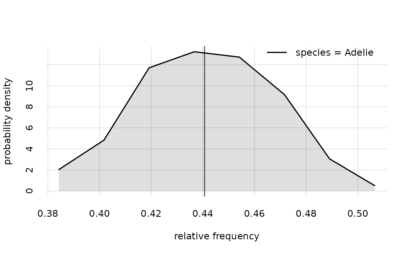
## Calculate the probability that an unknown penguin from this population
## is of species 'Adelie'
## more explicitly: Pr(Y = data.frame(species = 'Adelie'), K = Kexample)
probs <- Pr(data.frame(species = 'Adelie'), Kexample)
## display the probability value
probs$value
#>
#> species [,1]
#> Adelie 0.440685
## the full-population frequency of 'Adelie' penguins is unknown;
## display the 5.5%- and 94.5%-probability values
## for such frequency
probs$quantiles[, , c('5.5%', '94.5%')]
#> 5.5% 94.5%
#> 0.3988210 0.4829919
## we can also plot the probability distribution
## for this full-population frequency
hist(probs, legend = 'topright')
 ## ## Example 2:
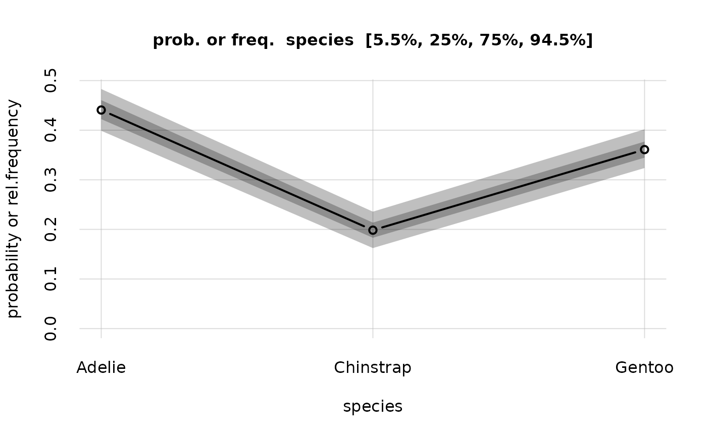
## Calculate the 3 probabilities that an unknown penguin from this population
## is of species 'Adelie', 'Chinstrap', 'Gentoo'
probs <- Pr(data.frame(species = c('Adelie', 'Chinstrap', 'Gentoo')),
Kexample)
## display the 3 probability values
probs$value
#>
#> species [,1]
#> Adelie 0.4406850
#> Chinstrap 0.1984161
#> Gentoo 0.3608989
## the full-population frequencies of the three species are unknown;
## display the 5.5%- and 94.5%-probability values
## for such frequencies
probs$quantiles[, , c('5.5%', '94.5%')]
#> Q
#> species 5.5% 94.5%
#> Adelie 0.3988210 0.4829919
#> Chinstrap 0.1623616 0.2357522
#> Gentoo 0.3237028 0.4017671
## plot the probabilities and quantiles
plot(probs)
## ## Example 2:
## Calculate the 3 probabilities that an unknown penguin from this population
## is of species 'Adelie', 'Chinstrap', 'Gentoo'
probs <- Pr(data.frame(species = c('Adelie', 'Chinstrap', 'Gentoo')),
Kexample)
## display the 3 probability values
probs$value
#>
#> species [,1]
#> Adelie 0.4406850
#> Chinstrap 0.1984161
#> Gentoo 0.3608989
## the full-population frequencies of the three species are unknown;
## display the 5.5%- and 94.5%-probability values
## for such frequencies
probs$quantiles[, , c('5.5%', '94.5%')]
#> Q
#> species 5.5% 94.5%
#> Adelie 0.3988210 0.4829919
#> Chinstrap 0.1623616 0.2357522
#> Gentoo 0.3237028 0.4017671
## plot the probabilities and quantiles
plot(probs)
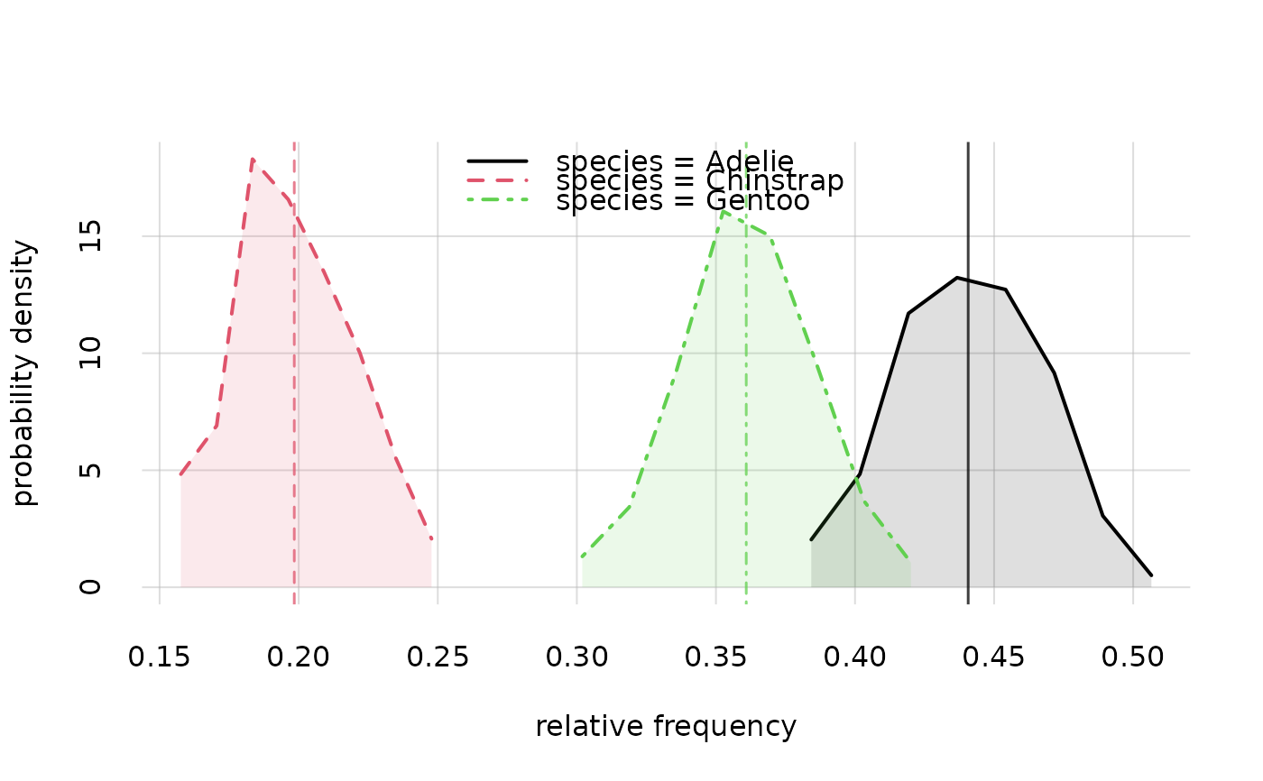
 ## plot the probability distribution for the full-population frequency
## of each species
hist(probs)
## plot the probability distribution for the full-population frequency
## of each species
hist(probs)
 ## ## Example 3:
## Calculate the probability that an unknown penguin is of species 'Adelie'
## GIVEN that its bill length is 43 mm
## more explicitly: Pr(Y = ..., X = ..., K = Kexample)
probs <- Pr(data.frame(species = 'Adelie'), data.frame(bill_len = 43),
Kexample)
## display the probability value
probs$value
#> |bill_len
#> species 43
#> Adelie 0.4647433
## the full-subpopulation frequency of 'Adelie' penguins,
## among penguins having bill length of 43 mm, is unknown;
## display the 5.5%- and 94.5%-probability values
## for such conditional frequency
probs$quantiles[, , c('5.5%', '94.5%')]
#> 5.5% 94.5%
#> 0.3669249 0.5678666
## ## Example 4:
## Calculate the probability that
## an unknown penguin is of species 'Adelie' AND its bill length is 43 mm
probs <- Pr(data.frame(species = 'Adelie', bill_len = 43), Kexample)
## display the probability value
probs$value
#>
#> species,bill_len [,1]
#> Adelie,43 0.001819114
## display the 5.5%- and 94.5%-probability values
## for the full-population frequency of 'Adelie' penguins with 43 mm bills
probs$quantiles[, , c('5.5%', '94.5%')]
#> 5.5% 94.5%
#> 0.001245039 0.002371801
## ## Example 5:
## Calculate the 3 x 2 probabilities for the 3 species
## GIVEN bill-lengths of 43 mm and 44 mm
Y <- data.frame(species = c('Adelie', 'Chinstrap', 'Gentoo'))
X <- data.frame(bill_len = c(43, 44))
probs <- Pr(Y, X, Kexample)
## display the 3 x 2 probability values
probs$value
#> |bill_len
#> species 43 44
#> Adelie 0.4647433 0.2223224
#> Chinstrap 0.1458345 0.2054491
#> Gentoo 0.3894222 0.5722285
## display the 5.5%- and 94.5%-probability values
## for the full-population joint frequencies
probs$quantiles[, , c('5.5%', '94.5%')]
#> , , Q = 5.5%
#>
#> |bill_len
#> species 43 44
#> Adelie 0.36692485 0.1447719
#> Chinstrap 0.08096214 0.1197566
#> Gentoo 0.29852092 0.4671262
#>
#> , , Q = 94.5%
#>
#> |bill_len
#> species 43 44
#> Adelie 0.5678666 0.3069388
#> Chinstrap 0.2190872 0.2965559
#> Gentoo 0.4811995 0.6718201
#>
## plot the probabilities and quantiles
plot(probs)
## ## Example 3:
## Calculate the probability that an unknown penguin is of species 'Adelie'
## GIVEN that its bill length is 43 mm
## more explicitly: Pr(Y = ..., X = ..., K = Kexample)
probs <- Pr(data.frame(species = 'Adelie'), data.frame(bill_len = 43),
Kexample)
## display the probability value
probs$value
#> |bill_len
#> species 43
#> Adelie 0.4647433
## the full-subpopulation frequency of 'Adelie' penguins,
## among penguins having bill length of 43 mm, is unknown;
## display the 5.5%- and 94.5%-probability values
## for such conditional frequency
probs$quantiles[, , c('5.5%', '94.5%')]
#> 5.5% 94.5%
#> 0.3669249 0.5678666
## ## Example 4:
## Calculate the probability that
## an unknown penguin is of species 'Adelie' AND its bill length is 43 mm
probs <- Pr(data.frame(species = 'Adelie', bill_len = 43), Kexample)
## display the probability value
probs$value
#>
#> species,bill_len [,1]
#> Adelie,43 0.001819114
## display the 5.5%- and 94.5%-probability values
## for the full-population frequency of 'Adelie' penguins with 43 mm bills
probs$quantiles[, , c('5.5%', '94.5%')]
#> 5.5% 94.5%
#> 0.001245039 0.002371801
## ## Example 5:
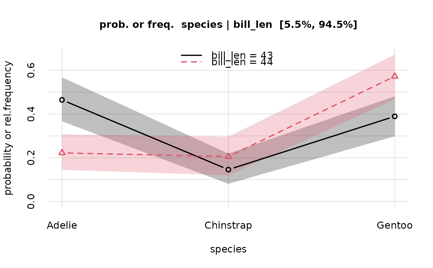
## Calculate the 3 x 2 probabilities for the 3 species
## GIVEN bill-lengths of 43 mm and 44 mm
Y <- data.frame(species = c('Adelie', 'Chinstrap', 'Gentoo'))
X <- data.frame(bill_len = c(43, 44))
probs <- Pr(Y, X, Kexample)
## display the 3 x 2 probability values
probs$value
#> |bill_len
#> species 43 44
#> Adelie 0.4647433 0.2223224
#> Chinstrap 0.1458345 0.2054491
#> Gentoo 0.3894222 0.5722285
## display the 5.5%- and 94.5%-probability values
## for the full-population joint frequencies
probs$quantiles[, , c('5.5%', '94.5%')]
#> , , Q = 5.5%
#>
#> |bill_len
#> species 43 44
#> Adelie 0.36692485 0.1447719
#> Chinstrap 0.08096214 0.1197566
#> Gentoo 0.29852092 0.4671262
#>
#> , , Q = 94.5%
#>
#> |bill_len
#> species 43 44
#> Adelie 0.5678666 0.3069388
#> Chinstrap 0.2190872 0.2965559
#> Gentoo 0.4811995 0.6718201
#>
## plot the probabilities and quantiles
plot(probs)
 ## ## Example 6:
## Calculate the 3 x 2 joint probabilities for the 3 species
## AND bill-lengths of 43 mm and 44 mm
Y <- expand.grid(
species = c('Adelie', 'Chinstrap', 'Gentoo'),
bill_len = c(43, 44)
)
probs <- Pr(Y, Kexample)
## display the 6 joint-probability values
probs$value
#>
#> species,bill_len [,1]
#> Adelie,43 0.0018191137
#> Chinstrap,43 0.0005712174
#> Gentoo,43 0.0015231253
#> Adelie,44 0.0009554396
#> Chinstrap,44 0.0008826070
#> Gentoo,44 0.0024593339
## display the 5.5%- and 94.5%-probability values
## for the full-population joint frequencies
probs$quantiles[, , c('5.5%', '94.5%')]
#> Q
#> species,bill_len 5.5% 94.5%
#> Adelie,43 0.0012450391 0.002371801
#> Chinstrap,43 0.0003027243 0.000897585
#> Gentoo,43 0.0010682562 0.002025675
#> Adelie,44 0.0005600381 0.001361621
#> Chinstrap,44 0.0004820964 0.001288832
#> Gentoo,44 0.0017899847 0.003151722
## ## Example 6:
## Calculate the 3 x 2 joint probabilities for the 3 species
## AND bill-lengths of 43 mm and 44 mm
Y <- expand.grid(
species = c('Adelie', 'Chinstrap', 'Gentoo'),
bill_len = c(43, 44)
)
probs <- Pr(Y, Kexample)
## display the 6 joint-probability values
probs$value
#>
#> species,bill_len [,1]
#> Adelie,43 0.0018191137
#> Chinstrap,43 0.0005712174
#> Gentoo,43 0.0015231253
#> Adelie,44 0.0009554396
#> Chinstrap,44 0.0008826070
#> Gentoo,44 0.0024593339
## display the 5.5%- and 94.5%-probability values
## for the full-population joint frequencies
probs$quantiles[, , c('5.5%', '94.5%')]
#> Q
#> species,bill_len 5.5% 94.5%
#> Adelie,43 0.0012450391 0.002371801
#> Chinstrap,43 0.0003027243 0.000897585
#> Gentoo,43 0.0010682562 0.002025675
#> Adelie,44 0.0005600381 0.001361621
#> Chinstrap,44 0.0004820964 0.001288832
#> Gentoo,44 0.0017899847 0.003151722