Plot the revisability of an object of class "prova_pr" (probability) as a histogram

The posterior probabilities calculated with the Pr() function, and outputted as a "prova_pr" (probability) object, have an associated "revisability" that comes from the finite size of the data sample. This revisability can be interpreted in two ways:

• How the probabilities could change, if we collected a much larger (infinite) data sample, and how likely would such change be;

• The relative frequency of a particular variate value in the full (sampled and unsampled) population is unknown; we can quantify our uncertainty about this relative frequency with a probability distribution.

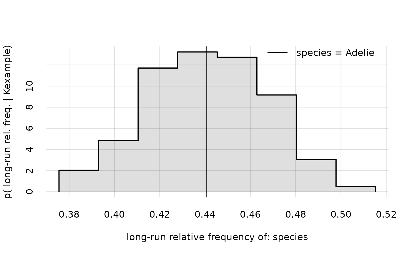
The hist() method for a "prova_pr" (probability) object is a utility to visualize this kind of revisability, in the form of a distribution. This distribution is represented by a histogram formed from samples of revised proobabilities (or long-run frequencies). The bin size is chosen according to the Monte Carlo accuracy.

Usage

# S3 method for class 'prova_pr'
hist(
  x,
  subset = NULL,
  breaks = NULL,
  legend = "topright",
  lty = c(1, 2, 4, 3, 6, 5),
  lwd = 2,
  col = palette(),
  alpha.f = 1,
  alpha.f.fill = 0.125,
  showmean = TRUE,
  xlab = NULL,
  ylab = NULL,
  xlim = NULL,
  ylim = c(0, NA),
  main = NULL,
  grid = TRUE,
  axes = FALSE,
  add = FALSE,
  ...
)

Arguments

x

Object of class "prova_pr" (probability), obtained with Pr().

subset

Named list or named vector: which variate values to display. For the variates corresponding to the names in this list, only the vector of values corresponding to that variate is displayed.

breaks

as in function graphics::hist(), or NULL (default). Value NULL determines bin width from the Monte Carlo accuracy (roughly speaking, each bin spans two standard deviations).

legend

One of the values "bottomright", "bottom", "bottomleft", "left", "topleft", "top", "topright", "right", "center" (see graphics::legend()): plot a legend at that position. A value FALSE or any other does not plot any legend. Default "top".

lty, lwd, col, alpha.f, xlab, ylab, xlim, ylim, main, grid, axes, add

see analogous arguments in graphics::matplot()

alpha.f.fill

Numeric, default 0.125: opacity of the histogram filling, 0 being completely invisible and 1 completely opaque.

showmean

Logical, default TRUE: show the means of the probability distributions? The means correspond to the probabilities about the next observed unit.

...

Other parameters to be passed to pplot().

Value

Invisibly, an object of class "histogram".

See also

Pr() to calculate posterior probabilities and quantiles.

plot.prova_pr() to plot the posterior probabilities.

pplot() (on which hist.prova_pr() is based) for more general plots.

Examples

## Use the "prova_K" (knowledge) object 'Kexample',
## calculated from the "penguins" dataset;
## variates: 'species' and 'bill_len'

## calculate the probability, and its revisability,
## for the value 'Adelie' of the "species" variate
probs <- Pr(data.frame(species = 'Adelie'), Kexample)
probs$value
#>         
#> species      [,1]
#>   Adelie 0.440685

## show the revisability of this probability; equivalently show
## the probability distribution for the relative frequency of
## 'Adelie' penguins in the full population
hist(probs, legend = 'topright')