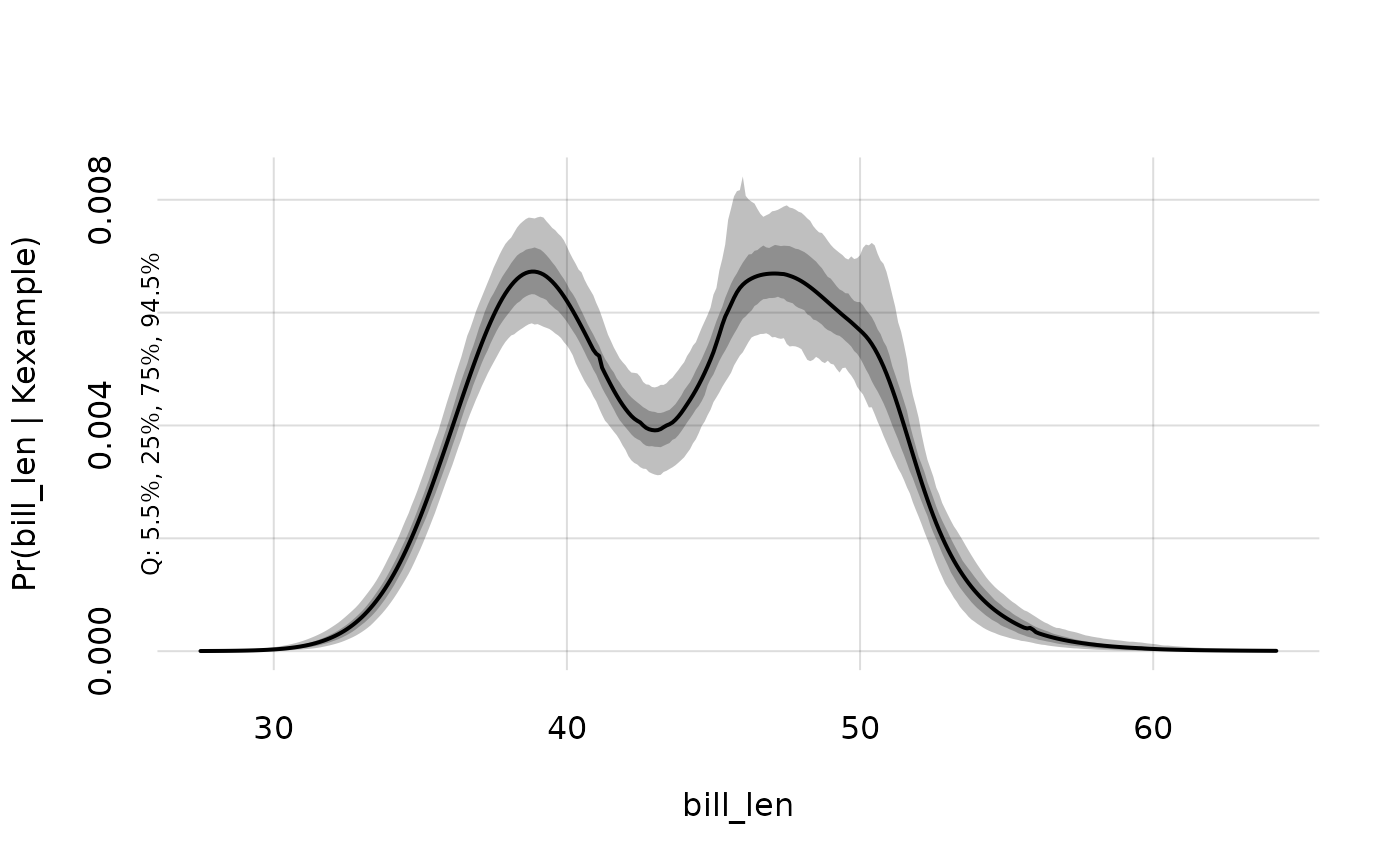
Plot an object of class "prova_pr" (probability)

This base::plot() method is a utility to plot probabilities obtained with Pr(), as well as their revisabilities. The probabilities are plotted either against Y, with one curve for each value of X, or vice versa.

Usage

# S3 method for class 'prova_pr'
plot(
  x,
  spread = NULL,
  subset = NULL,
  PvsY = NULL,
  type = NULL,
  lty = c(1, 2, 4, 3, 6, 5),
  pch = c(1, 2, 0, 5, 6, 3),
  lwd = 2,
  col = palette(),
  xlab = NULL,
  ylab = NULL,
  xlim = NULL,
  ylim = c(0, NA),
  legend = "topright",
  add = FALSE,
  alpha.f = 1,
  grid = TRUE,
  lwd.grid = NULL,
  col.grid = "#00000022",
  axes = FALSE,
  ylab2 = NULL,
  main = NULL,
  type.spread = NULL,
  lty.spread = 1,
  lwd.spread = NULL,
  alpha.f.spread = NULL,
  quantiles.spread = NULL,
  nsamples.spread = 360,
  ...
)

Arguments

x: Object of class "prova_pr" (probability), obtained with Pr().
spread: One of the values 'quantiles', 'samples', 'none' (equivalent to NA or FALSE), or NULL (default), in which case the revisability available in p is used. This argument chooses how to represent the revisability of the probability; see Pr(). If the requested representation is not available in the object x, then a warning is issued and no revisability is plotted.
subset: Named list or named vector: which variate values to display. For the variates corresponding to the names in this list, only the vector of values corresponding to that variate is displayed.
PvsY: Logical or NULL: should probabilities be plotted against their Y argument? If NULL, the argument between Y and X having larger number of values is chosen. As many probability curves will be plotted as the number of values of the other argument.
type: NULL (default) or character vector or list indicating the type of plot for the main probability distribution; see base::plot(). The default NULL value uses type 'l' (lines) for continuous variates, and 'b' (points and lines) for discrete variates.
lty: Analogous to argument lty (line style) in graphics::matplot(), used for the main probability distributions.
pch, col, xlab, ylab, main, xlim, ylim, grid, axes, add, lwd.grid, col.grid: see analogous arguments in graphics::plot.default() and graphics::matplot().
lwd: Analogous to argument lwd (line width) in graphics::matplot(), used for the main probability distributions.
legend: One of the values 'bottomright', 'bottom', 'bottomleft', 'left', 'topleft', 'top', 'topright', 'right', 'center' (see graphics::legend()): plot a legend at that position. A value FALSE or any other does not plot any legend. Default 'topright'.
alpha.f: Numeric, default 1: opacity of the colours of lines or markers, 0 being completely invisible and 1 completely opaque.
ylab2: A title for the y-axis on the right side of the plot, if displayed.
type.spread: NULL (default) or character vector or list indicating the type of plot for the long-run-frequency samples; see. The default NULL value uses type 'l' (lines) for continuous variates, and 'b' (points and lines) for discrete variates.
lty.spread: Same as parameter lty (line style), but for the line type of the long-run-frequency samples.
lwd.spread: Same as parameter lwd (line width), but for the line type of the long-run-frequency samples.
alpha.f.spread: Numeric or NULL (default): opacity of the quantile bands or of the long-run-frequency samples, similar to alpha.f. NULL means 0.25 if spread = 'quantiles'; and an appropriate value if spread = 'samples',dependent on the number of samples (more samples, less opacity).
quantiles.spread: Numeric vector or NULL (default): revisability quantiles to display. Value NULL uses all quantiles available in the x object, or just extreme quantiles if multiple probability curves are shown.
nsamples.spread: Integer, default 360: number of samples of long-run frequencies to display.
...: Other parameters to be passed to pplot().

Value

NULL, invisibly; produces a plot, see graphics::matplot().

Details

For a collection of probabilities \(\mathrm{Pr}(Y = y \vert X = x, K)\) with several values \(y\) and \(x\), this plot method with argument PvsY set to TRUE shows the probabilities on the y-axis, while the x-axis spans the \(y\) values, the curve thus showing the probability distribution (the area underneath is 1, except for possibly omitted tails). One such curve is displayed for each \(x\) value. If the argument PvsY is FALSE, then the x-axis spans the \(x\) values instead – thus the displayed curve is not a probability distribution (area underneath is not 1). One such curve is displayed for each \(y\) value. Which kind of plot is best depends on whether one needs to visualize how the probabilities depend on variate \(Y\) or on the conditioning variate \(X\). The default PvsY value NULL tries to guess the desider behaviour depending on how many different values \(y\) and \(x\) are contained in the probability object x; the variate with the largest number of values is displayed on the x-axis, so as to clutter as little as possible the plot window with multiple curves.

The revisabilities of the probabilities can be visualized in two different ways, determined by the argument spread:

spread = 'quantiles': shows the revisabilities as quantile bands around the probability curves. Which quantiles are shown depends on the quantiles.spread argument.
spread = 'samples': shows the revisabilities as an ensemble of alternative probability curves, which can also be interpreted as possible "long-run frequencies". The number of samples in the ensemble is determined by the argument nsamples.spread.
spread = 'none' or NA or FALSE: does not show any revisability.
spread = NULL (default): use the quantile plot, if quantiles are available; otherwise the ensemble plot, if samples are available; otherwise nothing.

Information about the revisability, such as quantiles or number of samples displayed, is shown beside the left y-axis. While quantile bands look neat, they do not show important details about revised probabilities (long-run frequencies), such as persistent modes. Such details are better displayed in the ensemble plot. It is recommended to always take a look at both visualizations of revisability.

The label on the left y-axis is by default the text Pr(\(Y\)|\(X\), \(K\)), displaying the actual \(Y\) and \(X\) variates present in the probability object x. If the displayed probabilities are densities (this means that some \(Y\) variates are continuous and not rounded), then lowercase p is used istead of Pr.

Continuous variates with bounded domains, such as censored variates, may have singular probability values – concentrated probability mass – at the boundary points. When such singular points are present, their probability scale is shown in the right y-axis.

Examples

## Use the "prova_K" (knowledge) object 'Kexample',
## calculated from the "penguins" dataset;
## variates: 'species' and 'bill_len'

## create a grid of values for variate "bill length",
## based on the information in the dataset and metadata:
valuesBill <- vrtgrid('bill_len', Kexample)

## calculate the probabilities and quantiles
probs <- Pr(valuesBill, Kexample)

## plot the probabilities and quantiles
plot(probs)