Plot numeric or character values

Plot function that modifies and expands the graphics package's graphics::matplot() function in several ways.

Usage

flexiplot(
  x,
  y,
  type = NULL,
  lty = c(1, 2, 4, 3, 6, 5),
  lwd = 2,
  pch = c(1, 2, 0, 5, 6, 3),
  col = palette(),
  xlab = NULL,
  ylab = NULL,
  xlim = NULL,
  ylim = NULL,
  add = FALSE,
  xdomain = NULL,
  ydomain = NULL,
  alpha.f = 1,
  xjitter = NULL,
  yjitter = NULL,
  grid = TRUE,
  cex.main = 1,
  ...
)

Arguments

x

Numeric or character: vector of x-coordinates. If missing, a numeric vector 1:... is created having as many values as the rows of y.

y

Numeric or character: vector of y coordinates. If missing, a numeric vector 1:... is created having as many values as the rows of x.

type, lty, lwd, pch, col, xlab, ylab, add, cex.main

see analogous arguments in graphics::matplot().

xlim, ylim

NULL (default) or a vector of two values. In the latter case, if any of the two values is not finite (including NA or NULL), then the min or max x- or y-coordinates of the plotted points are used.

xdomain, ydomain

Character or numeric or NULL (default): vector of possible values of the variables represented in the x- and y-axes, in case the x or y argument is a character vector. The ordering of the values is respected. If NULL, then unique(x) or unique(y) is used.

alpha.f

Numeric, default 1: opacity of the colours, 0 being completely invisible and 1 completely opaque.

xjitter, yjitter

Logical or NULL (default): add base::jitter() to x- or y-values? Useful when plotting discrete variates. If NULL, jitter is added if the values are of character (or factor) class.

grid

Logical: whether to plot a light grid. Default TRUE.

...

Other parameters to be passed to graphics::matplot().

Value

NULL, invisibly; produces a plot, see graphics::matplot().

Details

This function is essentially a wrapper around graphics::matplot(), augmenting the latter with some additional features useful for plotting data and results handled by Prova. Some of the additional features provided by flexiplot are the following:

• Either or both x and y arguments can be of class base::character. In this case, axes labels corresponding to the unique values are used (see arguments xdomain and ydomain). This makes it easier to plot nominal and ordinal variates.

• A jitter can also be added to the generated points, via the xjitter and yjitter switches. This makes it easier to generate scatter plots of nominal and ordinal variates.

• It is possible to specify only a lower or upper limit in the xlim and ylim arguments, letting the other limit to be found automatically. This can be useful in plotting probabilities, in cases where we want to specify the lower, 0 limit, but want the upper limit to simply be the the maximum probability.

• Transparency of lines or markers can be specified through argument alpha.f.

• The plotting style is different, and default argument type = 'l' (line plot) rather than type = 'p' (point plot).

See the package's vignettes for more examples.

See also

Pr() to calculate posterior probabilities and quantiles.

plot.probability() to directly plot posterior probabilities and quantiles contained in a probability object.

plotquantiles() to plot quantile ranges.

Examples

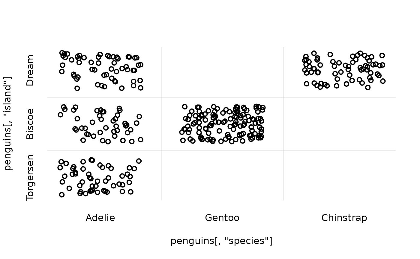
## Scatter plot of the 'island' vs 'species' nominal variates of the penguins dataset;
## note how jitter is automatically added:
flexiplot(x = penguins[, 'species'], y = penguins[, 'island'])



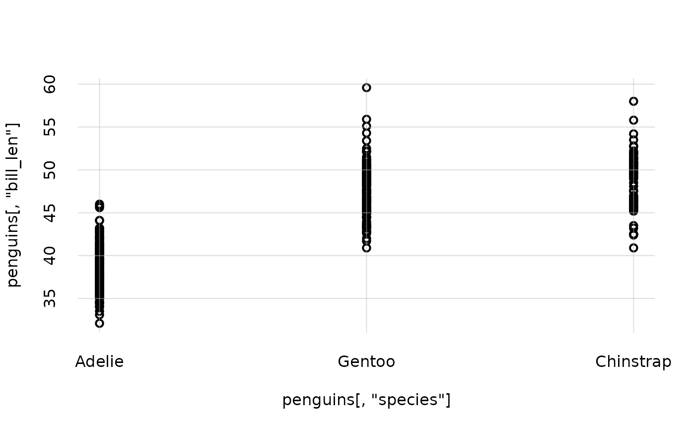
## Scatter plot of the 'bill_len' vs 'species' variates of the penguins dataset:
flexiplot(x = penguins[, 'species'], y = penguins[, 'bill_len'])


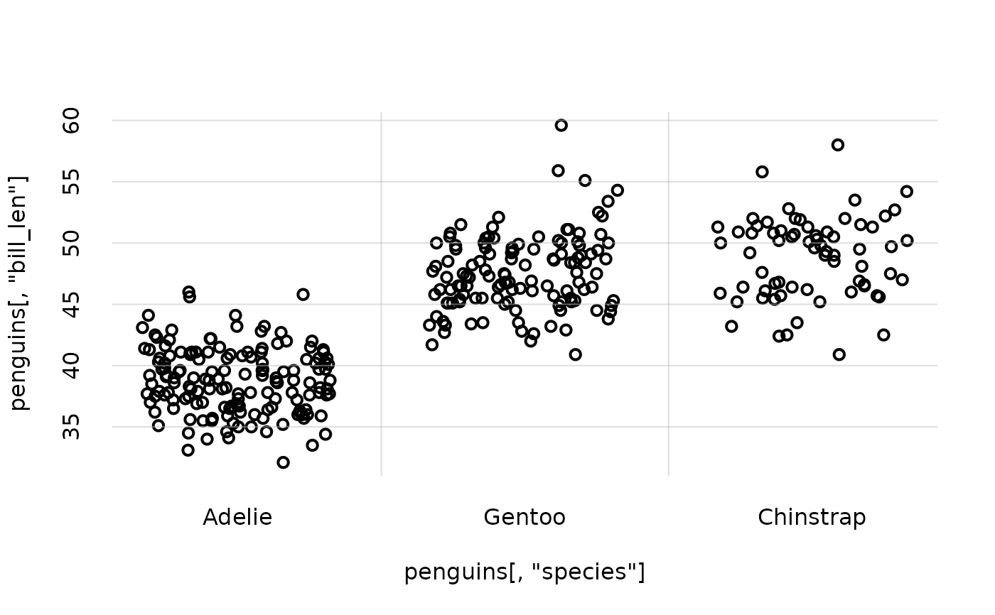
## We can add jitter to separate the nominal values:
flexiplot(x = penguins[, 'species'], y = penguins[, 'bill_len'],
  xjitter = TRUE)



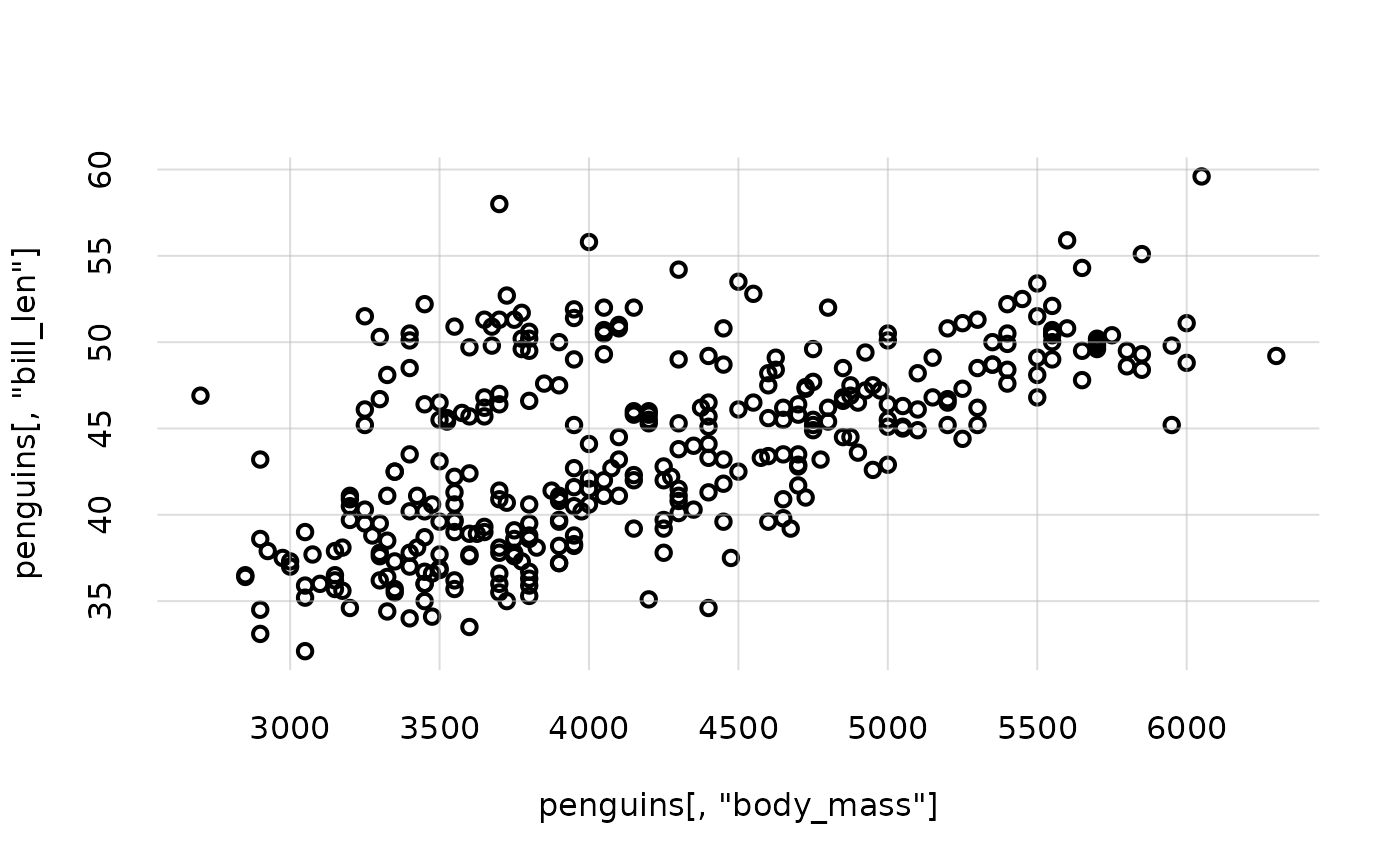
## Scatter plot of the 'bill_len' vs 'body_mass' variates;
## in this case we must specify the scatter-plot option `type = 'p'`:
flexiplot(x = penguins[, 'body_mass'], y = penguins[, 'bill_len'],
  type = 'p')


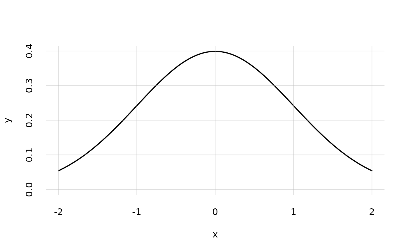
## Calculate the values of a normal distribution in a restricted range
x <- seq(from = -2, to = 2, length.out = 127)
y <- dnorm(x, mean = 0, sd = 1)

## plot the distribution, with 0 as the lower plot range:
flexiplot(x = x, y = y, ylim = c(0, NA))