Plot an object of class "probability"

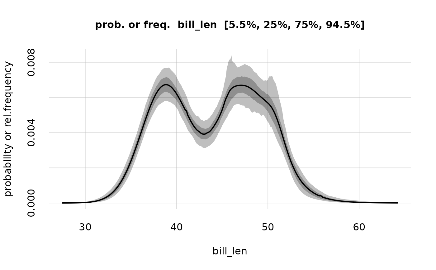
This base::plot() method is a utility to plot probabilities obtained with Pr(), as well as their revisabilities. The probabilities are plotted either against Y, with one curve for each value of X, or vice versa.

Usage

# S3 method for class 'probability'
plot(
  x,
  spread = NULL,
  subset = NULL,
  PvsY = NULL,
  legend = "topright",
  type = NULL,
  lty = c(1, 2, 4, 3, 6, 5),
  pch = c(1, 2, 0, 5, 6, 3),
  lwd = 2,
  col = palette(),
  xlab = NULL,
  ylab = NULL,
  xlim = NULL,
  ylim = c(0, NA),
  add = FALSE,
  alpha.f = 1,
  grid = TRUE,
  lwd.grid = NULL,
  col.grid = "#00000022",
  axes = FALSE,
  ylab2 = NULL,
  main = NULL,
  type.spread = NULL,
  lty.spread = c(1, 2, 4, 3, 6, 5),
  lwd.spread = NULL,
  alpha.f.spread = NULL,
  nsamples.spread = 360,
  ...
)

Arguments

x

Object of class "probability", obtained with Pr().

spread

One of the values 'quantiles', 'samples', 'none' (equivalent to NA or FALSE), or NULL (default), in which case the revisability available in p is used. This argument chooses how to represent the revisability of the probability; see Pr(). If the requested representation is not available in the object x, then a warning is issued and no revisability is plotted.

subset

Named list or named vector: which variate values to display. For the variates corresponding to the names in this list, only the vector of values corresponding to that variate is displayed.

PvsY

Logical or NULL: should probabilities be plotted against their Y argument? If NULL, the argument between Y and X having larger number of values is chosen. As many probability curves will be plotted as the number of values of the other argument.

legend

One of the values 'bottomright', 'bottom', 'bottomleft', 'left', 'topleft', 'top', 'topright', 'right', 'center' (see graphics::legend()): plot a legend at that position. A value FALSE or any other does not plot any legend. Default 'top'.

type

NULL (default) or character vector or indicating the type of plot for the main probability distribution; see base::plot(). The default NULL value uses type 'l' (lines) for continuous variates, and 'b' (points and lines) for discrete variates.

lty

Analogous to argument lty (line style) in graphics::matplot(), used for the main probability distributions.

pch, col, xlab, ylab, main, xlim, ylim, grid, axes, add, lwd.grid, col.grid

see analogous arguments in graphics::plot.default() and graphics::matplot().

lwd

Analogous to argument lwd (line width) in graphics::matplot(), used for the main probability distributions.

alpha.f

Numeric, default 1: opacity of the colours of lines or markers, 0 being completely invisible and 1 completely opaque.

ylab2

A title for the y-axis on the right side of the plot, if displayed.

type.spread

NULL (default) or character vector or indicating the type of plot for the long-run-frequency samples; see. The default NULL value uses type 'l' (lines) for continuous variates, and 'b' (points and lines) for discrete variates.

lty.spread

Same as parameter lty (line style), but for the line type of the long-run-frequency samples.

lwd.spread

Same as parameter lwd (line width), but for the line type of the long-run-frequency samples.

alpha.f.spread

Numeric or NULL (default): opacity of the quantile bands or of the long-run-frequency samples, similar to alpha.f. NULL means 1 if spread = 'samples' and 0.25 if spread = 'quantiles'.

nsamples.spread

Integer, default 360: number of samples of long-run frequencies to display.

...

Other parameters to be passed to pplot().

Value

NULL, invisibly; produces a plot, see graphics::matplot().

See also

Pr() to calculate posterior probabilities and quantiles.

hist.probability() to plot the revisability of the probabilities as a distribution.

pplot() (on which plot.probability() is based) for more general plots.

Examples

## Load the example `K`nowledge object calculated from the "penguins" dataset;
## variates: 'species' and 'bill_len'
K <- Kexample

## create a grid of values for variate "bill length",
## based on the information in the dataset and metadata:
valuesBill <- vrtgrid(vrt = 'bill_len', K = K)

## calculate the probabilities and quantiles
probs <- Pr(Y = valuesBill, K = K)

## plot the probabilities and quantiles
plot(probs)