Plot the revisability of an object of class "probability" as a histogram
Source:R/display.R
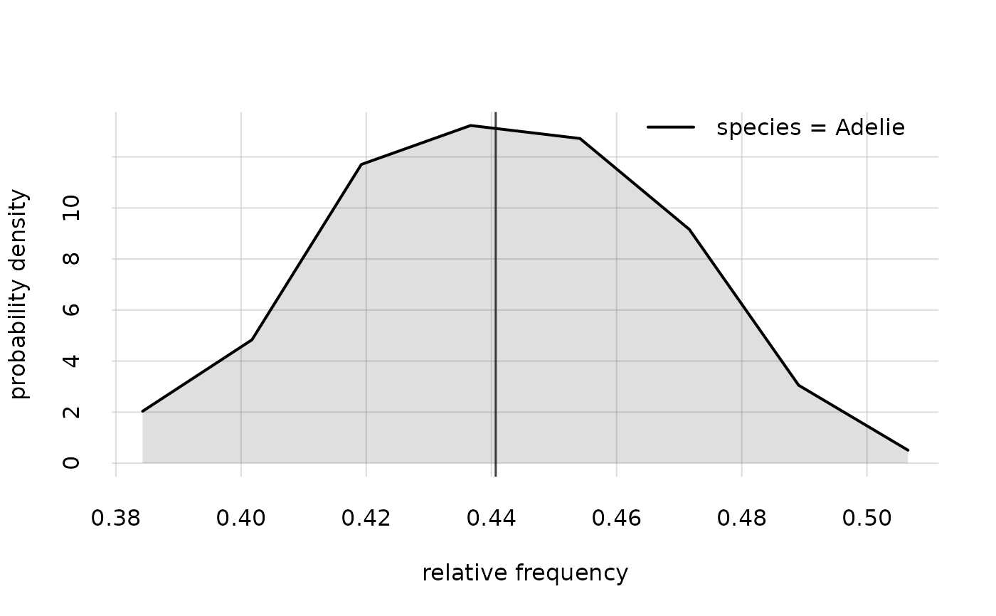
hist.probability.RdThe posterior probabilities calculated with the Pr() function, and outputted as a "probability" object, have an associated "revisability" that comes from the finite size of the data sample. This revisability can be interpreted in two ways:
How the probabilities could change, if we collected a much larger (infinite) data sample, and how likely would such change be;
The relative frequency of a particular variate value in the full (sampled and unsampled) population is unknown; we can quantify our uncertainty about this relative frequency with a probability distribution.
The hist() method for a "probability" object is a utility to visualize this kind of revisability, in the form of a distribution.
Usage
# S3 method for class 'probability'
hist(
  x,
  subset = NULL,
  breaks = NULL,
  legend = "topright",
  lty = c(1, 2, 4, 3, 6, 5),
  lwd = 2,
  col = palette(),
  alpha.f = 1,
  fill.alpha.f = 0.125,
  showmean = TRUE,
  xlab = NULL,
  ylab = NULL,
  xlim = NULL,
  ylim = c(0, NA),
  main = NULL,
  grid = TRUE,
  axes = FALSE,
  add = FALSE,
  ...
)
Arguments
- x
Object of class "probability", obtained with
Pr().- subset
Named list or named vector: which variate values to display. For the variates corresponding to the names in this list, only the vector of values corresponding to that variate is displayed.
- breaks
as in function
graphics::hist(), orNULL(default). ValueNULLuses the geometric mean of Sturges and Freedman-Diaconis bins.- legend
One of the values
"bottomright","bottom","bottomleft","left","topleft","top","topright","right","center"(seegraphics::legend()): plot a legend at that position. A valueFALSEor any other does not plot any legend. Default"top".- lty, lwd, col, alpha.f, xlab, ylab, xlim, ylim, main, grid, axes, add
see analogous arguments in
graphics::matplot()- fill.alpha.f
Numeric, default 0.125: opacity of the histogram filling.
0means no filling.- showmean
Logical, default
TRUE: show the means of the probability distributions? The means correspond to the probabilities about the next observed unit.- ...
Other parameters to be passed to
pplot().
Value
Invisibly, an object of class "histogram".
See also
Pr() to calculate posterior probabilities and quantiles.
plot.probability() to plot the posterior probabilities.
pplot() (on which hist.probability() is based) for more general plots.
Examples
## Load the example `K`nowledge object calculated from the "penguins" dataset;
## variates: 'species' and 'bill_len'
K <- Kexample

## calculate the probability, and its revisability,
## for the value 'Adelie' of the "species" variate
probs <- Pr(Y = data.frame(species = 'Adelie'), K = K)
probs$values
#>
#> species      [,1]
#>   Adelie 0.440685

## show the revisability of this probability; equivalently show
## the probability distribution for the relative frequency of
## 'Adelie' penguins in the full population
hist(probs, legend = 'topright')