Associations of variates with mutual information
Source:vignettes/vignette_mutualinfo.Rmd
vignette_mutualinfo.RmdBrief overview of the theory behind Mutual Information
Association and traditional measures for it
A probability quantifies our degree of belief in the values of some variates, given that we know the values of some other variates. This belief also reflect our uncertainty: maximal for a belief of 50%, minimal for a belief of 0% or 100%.
In some cases we wish to quantify our uncertainty in an average sense, rather than about specific values, or given knowledge of specific values. In other words, we ask: on average, how uncertain are we about a set of variates, given that we have knowledge of another set? If this average uncertainty is low, then we say that the two sets of variates are highly correlated or associated; otherwise, that the are uncorrelated. Here we are using the word ‘correlation’ in its general sense, not in the specific sense of “linear correlation” or similar.
Traditionally the Pearson correlation coefficient “” is used to quantify association. It is extremely limited, however. It is essentially based on the assumption that all variates involved have a joint Gaussian distribution. As a consequence, it is a measure of linear association, rather than general association. For instance, if the graph of two continuous variates and is a semicircle, then it means that is a function of , and is therefore perfectly associated with : if we know , then we can perfectly predict the value of . Yet the Pearson correlation coefficient between the two variates is in this case, simply because the functional dependence of on is not linear:
X <- seq(-1, 1, length.out = 200)
Y <- sqrt(1 - X^2)
r <- cor(X, Y, method = 'pearson')
plot(x = X, y = Y, type = 'p', main = paste0('Pearson correlation: ', signif(r, 2)))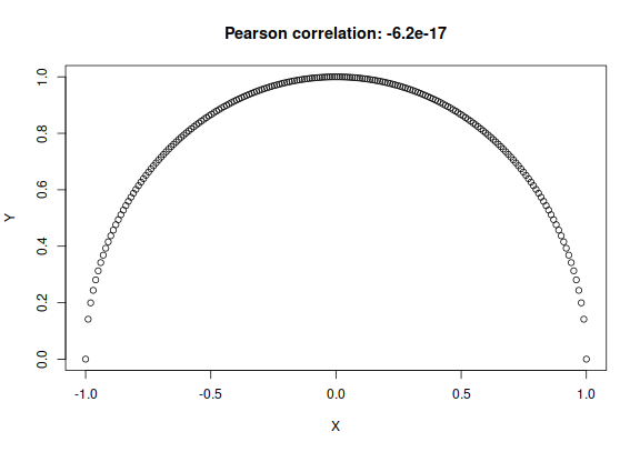
plot of chunk unnamed-chunk-1
Similar limitations of the Pearson correlation coefficient are demonstrated by the “Anscombe quartet” of datasets.
In the case of two variates, the limitations and possibly misleading value of the Pearson correlation coefficient may not be a serious problem, because we can visually inspect the relation and association between the variates. But in dealing with multi-dimensional variates, visualization is not possible and we must rely on the numerical values of the measure we use to quantify “association”. In such cases the Pearson correlation coefficient can be highly misleading, and let us conclude that there’s no association when actually there’s a very strong one. Considering that our world is highly non-linear, this possibility is far from remote.
Mutual Information
But there is a measure of association that does not suffer from the limitations discussed above: the mutual information between and . It has in fact the following important properties:
If there is no association whatever between and , in the sense that knowledge of one never changes our probabilities about the other, then the mutual information between them is zero. Vice versa, if the mutual information is zero, then there is no association whatever between and .
If and have a perfect association, that is, if knowing gives us perfect knowledge about or vice versa, or in yet other words if is a function of or vice versa, then the mutual information between them takes on its maximal possible value. Vice versa, if the mutual information takes on its maximal value, then one variate is a function of the other.
Regarding the last feature, note that the functional dependence between and can be of any kind, not just linear. This means that in the case of the semicircle plot above, the mutual information between and has its maximal value.
There’s also a special case in which the maximal value of the mutual information is zero, which indicates that is, technically speaking, a function of , yet knowledge of doesn’t give us any knowledge about . It’s the case where has just one value, independently of :
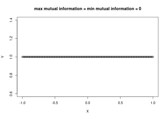
plot of chunk unnamed-chunk-2
Mutual information is measured in shannons (symbol ), or hartleys (symbol ), or natural units (symbol ). These units and other properties of the mutual information are standardized by the International Organization for Standardization (ISO) and the International Electrotechnical Commission (IEC). The minimum possible value of the mutual information is always zero. The maximum possible value depends instead on the variates and .
Interpretation of the values of mutual information
The value of the mutual information between two variates has an operational meaning and interpretation. To understand it we must first summarize the meaning of the Shannon information as a measure of uncertainty or of acquired information.
A value of shannons represents the uncertainty equivalent to not knowing which among possible alternatives is the true one. So represents the uncertainty between two equally possible cases, like the outcome of a coin toss. Other examples: represent being uncertain among 8 equally possible alternatives; represent being uncertain among 3 equally possible alternatives. If a clinician is uncertain about which disease, among four equally possible ones, affects a patient, then the clinician’s uncertainty is .
The “equivalence” in the definition above reflects the fact that some possibilities may have higher probabilities than others. For instance, if there are three alternatives but one of them has 0% probability, then our uncertainty is , the same as for two equally possible alternatives. If there are three possibilities with probabilities 11.4%, 11.4%, and 77.2%, then the uncertainty is approximately : as if there were only two alternatives; this is because one alternative has much higher probability than the other two.
Back to mutual information: If the mutual information between and amounts to , then knowledge of reduces, on average, times the number of uncertain possibilities of . For example, suppose that a clinician is uncertain about four possible diseases in a diagnosis (uncertainty of ), but there is a particular clinical indicator that associated with the disease. If the mutual information between the indicator and the disease is , then the clinician will be roughly uncertain about two possible diseases, rather than four, upon testing the clinical indicator. If the mutual information were instead, then the indicator would tell the disease with certainty.
You might think: “the value of mutual information is difficult to interpret”. But this is only a matter of getting familiar with it, by using it. Remember how difficult it was to get a feeling of what a particular value of the Pearson correlation really meant, when you first learned it. You developed an intuitive understanding of its range of values simply by using it. The same holds for mutual information.
For further discussion about mutual information and entropic measures of association, take a look at Information, relevance, independence, association and the references given there.
Function for the calculation of mutual information between variates
The software offers the function mutualinfo() to
calculate the mutual information between a set of joint variates
and another set
.
It requires at least three arguments:
-
Y1names: a vector the names (strings) of the variates in the first set; -
Y2names: a vector the names of the variates in the second set; -
learnt: the knowledge acquired from the dataset, calculated with thelearn()function.
It may be useful to specify two more arguments:
-
parallel: the number of CPUs to use for the computation; -
nsamples: the number of samples to use for the computation of the mutual information (default 3600).
The output of this function is a list of several entropic measures and other information. For this example we can focus on two outputs:
-
$MI: a vector of two numbers:valueis the value of the mutual information in shannons;erroris its numerical error (coming from the Monte Carlo calculation); -
$MImax: a vector of two numbers:valueis the value of the maximal possible value of the mutual information, in shannons;erroris its numerical error.
Example
As an example, let’s take the dataset and inference problem discussed in the vignette Example of use: inferences for Parkinson’s Disease.
Suppose we want to quantify the association between the treatment
group of a patient and the effect of the treatment. The treatment group
is given by the TreatmentGroup binary variate, and the
effect is quantified by the difference in MDS-UPDRS-III scores between
the first and second visits, in the variate
diff.MDS.UPRS.III. We use the knowledge calculated and
saved in the learnt.rds file.
The mutual information between TreatmentGroup and
diff.MDS.UPRS.III is
mutualinfoGroupEffect <- mutualinfo(
    Y1names = 'diff.MDS.UPRS.III',
    Y2names = 'TreatmentGroup',
    learnt = 'learnt.rds',
    parallel = 12
)
#>
#> Registered doParallelSNOW with 12 workers
#>
#> Closing connections to cores.

mutualinfoGroupEffect$MI
#>      value      error
#> 0.00182770 0.00105656

mutualinfoGroupEffect$MImax
#>        value        error
#> 1.0001446150 0.0000971804
The result is within the numerical error, out of a possible maximal value of around , shows that there is essentially no association between the treatment group and the effect. Note that further data could change this conclusion, though (the calculation of this uncertainty will be later implemented in the package).
We can also quantify the association between two sets of variates
within a subpopulation defined by a specific value of an
additional variate X (which may be a joint variate). This
subpopulation is specified by an additional argument X to
the mutualinfo() function. For instance, let’s quantify the
association between treatment group and effect within the subpopulation
of female patients only:
mutualinfoGroupEffectFemales <- mutualinfo(
    Y1names = 'diff.MDS.UPRS.III',
    Y2names = 'TreatmentGroup',
    X = data.frame(Sex = 'Female'),
    learnt = 'learnt.rds',
    parallel = 12
)
#>
#> Registered doParallelSNOW with 12 workers
#>
#> Closing connections to cores.

mutualinfoGroupEffectFemales$MI
#>      value      error
#> 0.00194501 0.00118147

mutualinfoGroupEffectFemales$MImax
#>       value       error
#> 0.999625276 0.000198657
The resulting mutual information is above zero, within twice the numerical error. So there’s a slightly larger – though still extremely weak – association between the treatment group and effect within the female subpopulation.
(TO BE CONTINUED)