Example of use: inferences for Parkinson's Disease
Source:vignettes/vignette_parkinson.Rmd
vignette_parkinson.RmdPurpose
Here is a toy example showing some kinds of results that can be obtained with Bayesian nonparametric exchangeable inference. The example involves inferences about some investigations on Parkinson’s Disease described in the paper by Brakedal & al. (2022), which generously and professionally shares its data.
The investigations in the cited paper involve 30 subjects, for each
of which various data are collected. Fifteen of these subjects belong to
a control group, the other 15 to the treatment group, denoted
NR. This group received a nicotinamide adenine dinucleotide
(NAD) replenishment therapy, via oral intake of nicotinamide riboside
(NR). In this toy example we do not follow or reproduce the paper’s
investigations, nor do we use all the variates observed. We limit
ourselves to 7 variates for each subject. Here is a list with a brief
description of each:
Treatment group: Binary variate with values
PlaceboandNR.Sex: Binary variate with values
FemaleandMale.Age: Integer variate, or continuous but rounded variate.
Anamnestic loss of smell: Binary variate with values
NoandYes.History of REM sleep behaviour disorder: Binary variate with values
NoandYes.MDS-UPDRS-III score at the first subject visit: The MDS-UPDRS-III (Movement Disorder Society’s Unified Parkinson’s Disease Rating Scale) is one of a set of ordinal scales to assess a subject’s degree of disability and monitor it over time. The scale III ranges from
0(no disability) to132(highest degree of disability). Given that operations such as sum or average are performed on these scales in the literature, the scales should be considered on an interval kind rather than simply ordinal.Difference in MDS-UPDRS-III scores between second and first visit: Ordinal variate, the difference of the previous one between the subject’s second and first visit. Its range is therefore from
-132to+132, negative values representing an improvement.
We store the name of the datafile
datafile <- 'toydata.csv'Here are the values for two subjects:
| TreatmentGroup | Sex | Age | Anamnestic.Loss.of.smell | History.of.REM.Sleep.Behaviour.Disorder | MDS.UPDRS..Subsection.III.V1 | diff.MDS.UPRS.III |
|---|---|---|---|---|---|---|
| Placebo | Male | 66 | No | No | 44 | -2 |
| NR | Female | 65 | Yes | No | 32 | 10 |
“Natural” vs controlled or “biased” variates
For the purpose of drawing scientific inferences, it is extremely important to be mindful of which variates in the dataset have “natural” statistics, and which instead have statistics controlled by the observer – and are therefore “biased”. This distinction is important because the dataset statistics of the controlled variates may then not be representative of the naturally-occurring ones, and therefore cannot be used for inference purposes.
In the present dataset, for instance, the numbers of
Placebo and NR subjects were decided by the
investigators to be in a 50%/50% proportion. Obviously this is not a
naturally occurring proportion; in fact, it does not even make sense of
speaking of a naturally occurring statistics for this
TreatmentGroup variate.
For the Sex variate, the dataset has a proportion of
around 17% Female and 83% Male subjects. This
proportion also partly stems from the selection procedure of the
investigators, so we cannot infer that roughly 16% of Parkinson patients
in the national population are females. It is also possible that the
proportions in the Age variate may depend on the selection
procedure.
On the other hand, the investigators did not choose the
statistics of the two MDS.UPDRS variates, within the groups
having particular values of the other variates. This
conditional or subpopulation statistics can be taken
as representatives of naturally-occurring ones (see Lindley & Novick
(1980) for a brilliant discussion of this point).
(add short explanation of exchangeability)
Metadata
Let’s load the package:
In order to draw inferences, we need metadata information, that is, information about the variates that is not present in the data. Such information mainly regard the kind and domain of each variate.
As an example of why metadata is necessary, suppose you are given the
data 3, 7, 9. Can you say whether
the value 5 could be observed in a new instance? and what
about 4.7, or -10? Knowing whether these
values are at all possible, or not, greatly affects the precision of the
inferences we draw. Obviously a researcher must know such basic
information about the data being collected – otherwise they wouldn’t
know what they’re doing.
The software requires specification of metadata either as a
data.frame object or as a .csv file. To help
you prepare this file, the software offers the function
metadatatemplate(), which writes a template that you
thereafter modify. The template is filled with
tentative values; these are wild guesses from the data,
so they are often wrong. The function explains the heuristic it is using
in order to pre-fill the fields of the metadata file, and gives warnings
about guessed values that are especially dubious. You should examine and
correct all fields:
metadatatemplate(data = datafile, file = 'temp_metadata')
#>
#> Analyzing 7 variates for 30 datapoints.
#>
#> * "TreatmentGroup" variate:
#>   -  2 different  values detected:
#>  "NR", "Placebo"
#>   which do not seem to refer to an ordered scale.
#>   Assuming variate to be NOMINAL.
#>
#> * "Sex" variate:
#>   -  2 different  values detected:
#>  "Female", "Male"
#>   which do not seem to refer to an ordered scale.
#>   Assuming variate to be NOMINAL.
#>
#> * "Age" variate:
#>   - Numeric values between 29 and 75
#>   Assuming variate to be CONTINUOUS.
#>   - Distance between datapoints is a multiple of 1
#>   Assuming variate to be ROUNDED.
#>   - All values are positive
#>   Assuming "domainmin" to be 0
#>
#> * "Anamnestic.Loss.of.smell" variate:
#>   -  2 different  values detected:
#>  "No", "Yes"
#>   which do not seem to refer to an ordered scale.
#>   Assuming variate to be NOMINAL.
#>
#> * "History.of.REM.Sleep.Behaviour.Disorder" variate:
#>   -  2 different  values detected:
#>  "No", "Yes"
#>   which do not seem to refer to an ordered scale.
#>   Assuming variate to be NOMINAL.
#>
#> * "MDS.UPDRS..Subsection.III.V1" variate:
#>   - Numeric values between 15 and 50
#>   Assuming variate to be CONTINUOUS.
#>   - Distance between datapoints is a multiple of 1
#>   Assuming variate to be ROUNDED.
#>   - All values are positive
#>   Assuming "domainmin" to be 0
#>
#> * "diff.MDS.UPRS.III" variate:
#>   - Numeric values between -9 and 10
#>   Assuming variate to be CONTINUOUS.
#>   - Distance between datapoints is a multiple of 1
#>   Assuming variate to be ROUNDED.
#> =========
#> WARNINGS - please make sure to check these variates in the metadata file:
#>
#> * "Age" variate appears to be continuous and rounded,
#> but it could also be an ordinal variate
#>
#> * "MDS.UPDRS..Subsection.III.V1" variate appears to be continuous and rounded,
#> but it could also be an ordinal variate
#>
#> * "diff.MDS.UPRS.III" variate appears to be continuous and rounded,
#> but it could also be an ordinal variate
#> =========
#>
#> Saved proposal metadata file as "temp_metadata.csv"
We can open the temporary metadata file
temp_metadata.csv and edit it with any software of our
choice. Let’s save the corrected version as
meta_toydata.csv:
metadatafile <- 'meta_toydata.csv'The metadata are as follows; NA indicate empty
fields:
| name | type | datastep | domainmin | domainmax | minincluded | maxincluded | V1 | V2 |
|---|---|---|---|---|---|---|---|---|
| TreatmentGroup | nominal | NR | Placebo | |||||
| Sex | nominal | Female | Male | |||||
| Age | continuous | 1 | 0 | |||||
| Anamnestic.Loss.of.smell | nominal | No | Yes | |||||
| History.of.REM.Sleep.Behaviour.Disorder | nominal | No | Yes | |||||
| MDS.UPDRS..Subsection.III.V1 | ordinal | 1 | 0 | 132 | yes | yes | ||
| diff.MDS.UPRS.III | ordinal | 1 | -132 | 132 | yes | yes |
For a description of the metadata fields, see the help for
metadata with ?inferno::metadata.
(More to be written here!)
Learning
Our inferences will be based on the data already observed, and will mainly take the form of probabilities about the unkonwn values various quantities , given the observed values of other quantities : As the notation above indicates, these probabilities also depend on the already observed. They are usually called “posterior probabilities”.
We need to prepare the software to perform calculations of posterior
probabilities given the observed data. In machine learning an analogous
process is called “learning”. For this reason the function that achieves
this is called learn(). It requires at least three
arguments:
-
data, which can be given as a path to thecsvfile containing the data -
metadata, which can also be given as a path to the metadata file -
outputdir: the name of the directory where the output should be saved.
It may be useful to specify two more arguments:
-
seed: the seed for the random-number generator, to ensure reproducibility -
parallel: the number of CPUs to use for the computation
Alternatively you can set the seed with set.seed(), and
start a set of parallel workers with the
parallel::makeCluster() and
doParallel::registerDoParallel() commands.
The “learning” computation can take tens of minutes, or hours, or
even days depending on the number of variates and data in your inference
problem. The learn() function outputs various messages on
how the computation is proceeding. As an example:
learnt <- learn(
    data = datafile,
    metadata = metadatafile,
    outputdir = 'parkinson_computations',
    seed = 16,
    parallel = 12)

#> Registered doParallelSNOW with 12 workers
#>
#> Using 30 datapoints
#> Calculating auxiliary metadata
#>
#> **************************
#> Saving output in directory
#> parkinson_computations
#> **************************
#> Starting Monte Carlo sampling of 3600 samples by 60 chains
#> in a space of 703 (effectively 6657) dimensions.
#> Using 12 cores: 60 samples per chain, 5 chains per core.
#> Core logs are being saved in individual files.
#>
#> C-compiling samplers appropriate to the variates (package Nimble)
#> this can take tens of minutes with many data or variates.
#> Please wait...
At the end of the computation the learn() function
returns the name of the directory in which the results are saved. In the
code snipped above, this name is saved in the variable
learnt. The object containing the information needed to
make inferences is the learnt.rds file within this
directory.
Drawing inferences
We are finally ready to use the software for drawing inferences, testing hypotheses, and similar scientific investigations. From the observed data, the software allows us to find the probability of any question or hypothesis of interest. It is important, though, that the hypothesis be stated in an unambiguous, quantitative form.
First example: effect on treated patient of female sex
For example, we might want to ask: “Does the NAD-replenishment therapy have an effect on females?”. At first this may sound like a valid scientific hypothesis. But if we carefully examine the statement we realize that it is too vague. First, what does “having an effect” mean exactly? how can this be quantified? Second, can we really say that the therapy either has or has not an effect? are there no degrees of efficacy involved? Third, whom are we asking this question about? the next patient that we may see? or the population of all the remaining patients? Let us make our initial question quantitatively clear.
First, let us translate “effect” into the difference in MDS-UPDRS-III
scores between the first and second visits of a subject
(visit 2
visit 1), represented by the variate diff.MDS.UPRS.III.
Note that other choices could be made, such as the difference in another
MDS-UPDRS score (I–IV), or in the total of these scores, or as the ratio
rather than the difference – or as some other variate altogether.
Second, instead of asking the unrealistic dichotomous question “has or has not?”, we ask how strong the effect is, as quantified by the value of the MDS-UPDRS-III decrease.
Third, let us ask this question about a possible next patient. We shall see that this question is also related to the population as a whole.
We can calculate the probability that, in the next patient, we shall observe any particular value of the MDS-UPDRS-III difference, given that the patient is Female, and given what has been observed in the clinical trials:
The function for this is Pr(Y, X, learnt), which accepts
three arguments:
-
Y: the variates and values of which we want the probability -
X: the variates and values which are known -
learnt: the knowledge acquired from the dataset
Let us first ask this for a specific value of the MDS-UPDRS-III
difference, let’s say 0:
probability0 <- Pr(
    Y = data.frame(diff.MDS.UPRS.III = 0),
    X = data.frame(Sex = 'Female', TreatmentGroup = 'NR'),
    learnt = learnt
)
The output of the Pr() function is a list of several
objects, of which we discuss only two for the moment:
-
value: this is the value of the probability we wanted to know. In this case it is
probability0$value
#>       X
#> Y          [,1]
#>   [1,] 0.064202
that is, there is approximately a 6.4% probability that the next treated female patient will have a MDS-UPDRS-III difference of exactly 0.
-
quantiles: these values tell us how much the probability could change, if our knowledge were updated by more clinical trials. They thus quantify the uncertainty of our present probabilistic conclusions. A future, updated probability has a 89% probability of lying between the two extreme (5.5% and 94.5%) quantile values, and a 50% probability of lying between the middle (25% and 75%) ones q(these are typical intervals used in the Bayesian literature, see for instance Makowski et al.). In this case they are
probability0$quantiles
#> , ,  = 5.5%
#>
#>       X
#> Y           [,1]
#>   [1,] 0.0289361
#>
#> , ,  = 25%
#>
#>       X
#> Y           [,1]
#>   [1,] 0.0448123
#>
#> , ,  = 75%
#>
#>       X
#> Y          [,1]
#>   [1,] 0.077569
#>
#> , ,  = 94.5%
#>
#>       X
#> Y          [,1]
#>   [1,] 0.111913
that is, if we had many more clinical trials, the probability above could change to a value within around 2.9% and 11%.
We can obviously also ask for the probabilities of all possible values that the MDS-UPDRS-III difference could have in the next treated female patient:
probabilities <- Pr(
    Y = data.frame(diff.MDS.UPRS.III = (-30):30),
    X = data.frame(Sex = 'Female', TreatmentGroup = 'NR'),
    learnt = learnt
)
Each probability thus obtained has two accompanying quantiles and
related uncertainty. Both can be visualized with the plot()
function:
plot(probabilities)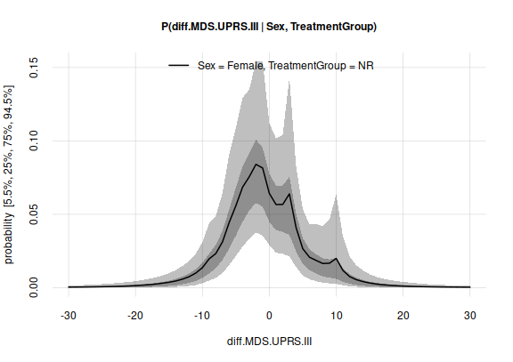
plot of chunk unnamed-chunk-13
Two aspects of this plot are relevant for our investigation:
There seems to be slightly more probability mass towards negative MDS-UPDRS-III differences – which means an improvement in the degree of disability. We shall quantify this further in a moment.
However, it is also clear that further clinical trials could lead to a quite different probability distribution. This is shown by the breadth of the quantile range.
Another way to graphically represent and see potential variability of
the result if more trials were available, is to plot some examples – say
100 – of how the results could differ. Such examples are stored in the
third object, samples given by the Pr()
function:
plot(probabilities, variability = 'samples',
    ylim = c(0, max(probabilities$quantiles)) # keep same y-range as before
    )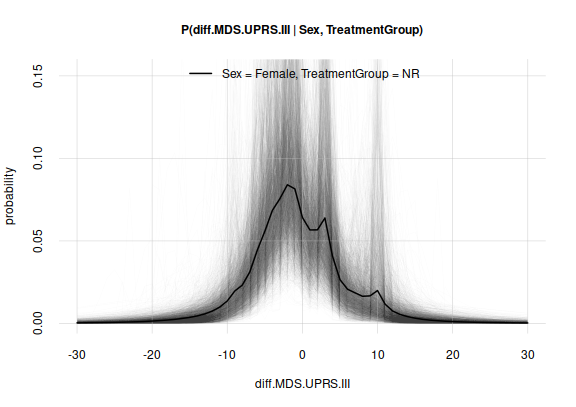
plot of chunk unnamed-chunk-14
Let us ask a more interesting question, which can be a quantitative counterpart of our initial question “Does the NAD-replenishment therapy have an effect on females?”. We ask: will the next treated female patient experience a MDS-UPDRS-III difference equal to or less?“. We therefore want the probability
This probability can be calculated with the function
tailPr(Y, X, learnt), which is analogous to the
Pr() function, but calculates the probability of
rather than of
.
probDecrease <- tailPr(
    Y = data.frame(diff.MDS.UPRS.III = -1),
    X = data.frame(Sex = 'Female', TreatmentGroup = 'NR'),
    learnt = learnt
)
The answer is that the probability of a decrease in this disability score is
probDecrease$value
#>       X
#> Y          [,1]
#>   [1,] 0.549769
or approximately 55%; note that it is clearly higher than 50%.
Further clinical trials, however could update this probability to a new value between 34% and 75%:
probDecrease$quantiles[1,1,]
#>     5.5%      25%      75%    94.5%
#> 0.342894 0.463976 0.641548 0.747442
Second example: comparison with non-treated patient of female sex
In the previous example we found that there is a 55% probability that a treated female patient will experience a decrease in MDS-UPDRS-III after the therapy. But can this decrease really be correlated with the therapy?
To preliminarily answer this question, we can find the analogous
probabilities for a female patient that has not received the treatment.
Again we use Pr(), but our X argument will
specify a Placebo value for the Treatment group:
probabilitiesPlacebo <- Pr(
    Y = data.frame(diff.MDS.UPRS.III = (-30):30),
    X = data.frame(Sex = 'Female', TreatmentGroup = 'Placebo'),
    learnt = learnt
)
Let’s plot these probabilities, together with their variability (only the most extreme case), on top of the ones previously obtained for the treated case:
plotquantiles(x = (-30):30, y = probabilities$quantiles[,1, c('5.5%', '94.5%')],
    ylim = c(0, NA),
    xlab = 'MDS-UPDRS-III difference', ylab = 'probability', col = 3)

plotquantiles(x = (-30):30, y = probabilitiesPlacebo$quantiles[,1, c('5.5%', '94.5%')],
    col = 2, add = TRUE)

flexiplot(x = (-30):30, y = probabilities$values[,1], col = 3, lwd = 2, add = TRUE)

flexiplot(x = (-30):30, y = probabilitiesPlacebo$values[,1],
    col = 2, lty = 2, add = TRUE)

## add 0-change line
abline(v = 0, lwd = 1, col = 5)

legend('topright', legend = c('NR, Female', 'Placebo, Female'),
    bty = 'n', lty = 1:2, col = 3:2)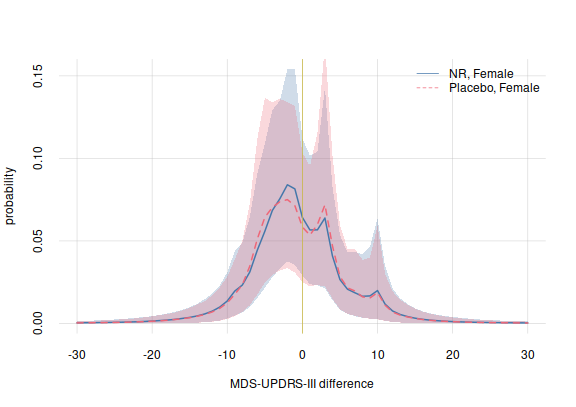
plot of chunk unnamed-chunk-20
There does not seem to be any difference that stands out between the treated and non-treated case.
As before, we can calculate the probability of a decrease in MDS-UPDRS-III:
probDecreasePlacebo <- tailPr(
    Y = data.frame(diff.MDS.UPRS.III = -1),
    X = data.frame(Sex = 'Female', TreatmentGroup = 'Placebo'),
    learnt = learnt
)
We find that the probability of a decrease in the disability score for a non-treated female patient is
probDecreasePlacebo$value
#>       X
#> Y          [,1]
#>   [1,] 0.543251
or approximately 54%. Further clinical trials, however could update this probability to a value between 33% and 74%:
probDecreasePlacebo$quantiles[1,1,]
#>     5.5%      25%      75%    94.5%
#> 0.333219 0.453890 0.632558 0.743401
Therefore we see a similarly probable decrease in a non-treated as well as a non-treated female patient. There is a very small difference in these two probabilities, in favour of the treated case; but this difference is too small compared with how the probabilities could change if more trials were available.
Some preliminary conclusions and possible questions for future research:
There does not seem to be a difference between treated and non-treated female patients, regarding MDS-UPDRS-III decrease.
However, there is a slightly likely decrease for both. What could this decrease be correlated with?
Third example: considering age
Our results so far indicate practically no difference in the probabilities of MDS-UPDRS-III decrease of a treated vs a non-treated female patient. These probabilities, however, disregard the patient’s age. Is it possible that there are larger differences in different age groups?
We can answer this question by calculating the probabilities
conditional on any particular Age value, that is,
for meaningful values
of the age, let’s say between 25 and 80. Again we can find them with the
function tailPr(). This time our conditioning argument
X will include a grid of Age values. First we
do the calculation for a treated female patient, then for a non-treated
one:
probDecreaseAge <- tailPr(
    Y = data.frame(diff.MDS.UPRS.III = -1),
    X = data.frame(Sex = 'Female', Age = 25:80, TreatmentGroup = 'NR'),
    learnt = learnt
)

probDecreaseAgePlacebo <- tailPr(
    Y = data.frame(diff.MDS.UPRS.III = -1),
    X = data.frame(Sex = 'Female', Age = 25:80, TreatmentGroup = 'Placebo'),
    learnt = learnt
)
We can plot the probabilities of an MDS-UPDRS-III decrease against that patient’s age, with one plot for each treatment group:
plotquantiles(x = 25:80, y = probDecreaseAge$quantiles[1,, c('5.5%', '94.5%')],
    ylim = c(0, NA),
    xlab = 'age', ylab = 'probability of MDS-UPDRS-III decr.', col = 3)

plotquantiles(x = 25:80, y = probDecreaseAgePlacebo$quantiles[1,, c('5.5%', '94.5%')],
    col = 2, add = TRUE)

flexiplot(x = 25:80, y = probDecreaseAge$values[1,], col = 3, lwd = 2, add = TRUE)

flexiplot(x = 25:80, y = probDecreaseAgePlacebo$values[1,],
    col = 2, lwd = 2, lty = 2, add = TRUE)

## add 50%-probability line
abline(h = 0.5, lwd = 1, col = 5)

legend('topright', legend = c('NR, Female', 'Placebo, Female'),
    bty = 'n', lty = 1:2, col = 3:2)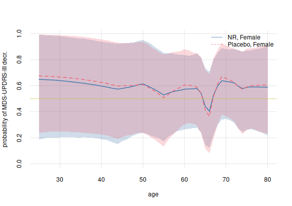
plot of chunk unnamed-chunk-25
This plot shows some interesting aspects:
There does not seem to be a large difference, between treated and non-treated females, in the probability of a MDS-UPDRS-III decrease.
In the 60–65 age group, an increase in MDS-UPDRS-III is more likely than a decrease, for both a treated and a non-treated female patient. What could be the reason for the increase in this narrow age group?
Again notice that these probabilities could be updated to very different values, if more clinical trials were available.
Fourth example: male patient
We can perform an analysis analogous to the previous examples, but for a male patient. Here are the corresponding function calls and plots.
probabilitiesMale <- Pr(
    Y = data.frame(diff.MDS.UPRS.III = (-30):30),
    X = data.frame(Sex = 'Male', TreatmentGroup = c('NR', 'Placebo')),
    learnt = learnt
)

plotquantiles(x = (-30):30, y = probabilitiesMale$quantiles[,1, c('5.5%', '94.5%')],
    ylim = c(0, NA),
    xlab = 'MDS-UPDRS-III difference', ylab = 'probability', col = 7)

plotquantiles(x = (-30):30, y = probabilitiesMale$quantiles[,2, c('5.5%', '94.5%')],
    col = 6, add = TRUE)

flexiplot(x = (-30):30, y = probabilitiesMale$values[,1],
    col = 7, lwd = 2, add = TRUE)

flexiplot(x = (-30):30, y = probabilitiesMale$values[,2],
    col = 6, lwd = 2, lty = 2, add = TRUE)

## add 0-change line
abline(v = 0, lwd = 1, col = 5)

legend('topright', legend = c('NR, Male', 'Placebo, Male'),
    bty = 'n', lty = 1:2, col = 7:6)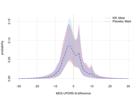
plot of chunk unnamed-chunk-26
And considering all ages separately:
probMaleDecreaseAge <- tailPr(
    Y = data.frame(diff.MDS.UPRS.III = -1),
    X = data.frame(Sex = 'Male', Age = 25:80, TreatmentGroup = 'NR'),
    learnt = learnt
)

probMaleDecreaseAgePlacebo <- tailPr(
    Y = data.frame(diff.MDS.UPRS.III = -1),
    X = data.frame(Sex = 'Male', Age = 25:80, TreatmentGroup = 'Placebo'),
    learnt = learnt
)


plotquantiles(x = 25:80, y = probMaleDecreaseAge$quantiles[1,, c('5.5%', '94.5%')],
    ylim = c(0, NA),
    xlab = 'age', ylab = 'probability of MDS-UPDRS-III decr.', col = 7)

plotquantiles(x = 25:80, y = probMaleDecreaseAgePlacebo$quantiles[1,, c('5.5%', '94.5%')],
    col = 6, add = TRUE)

flexiplot(x = 25:80, y = probMaleDecreaseAge$values[1,],
    col = 7, lwd = 2, add = TRUE)

flexiplot(x = 25:80, y = probMaleDecreaseAgePlacebo$values[1,],
    col = 6, lwd = 2, lty = 2, add = TRUE)

## add 50%-probability line
abline(h = 0.5, lwd = 1, col = 5)

legend('topright', legend = c('NR, Male', 'Placebo, Male'),
    bty = 'n', lty = 1:2, col = 7:6)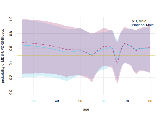
plot of chunk unnamed-chunk-27
Finally let’s compare treated female vs male patients, per age:
plotquantiles(x = 25:80, y = probDecreaseAge$quantiles[1,, c('5.5%', '94.5%')],
    ylim = c(0, NA),
    xlab = 'age', ylab = 'probability of MDS-UPDRS-III decr.', col = 3)

plotquantiles(x = 25:80, y = probMaleDecreaseAge$quantiles[1,, c('5.5%', '94.5%')],
    col = 7, add = TRUE)

flexiplot(x = 25:80, y = probDecreaseAge$values[1,],
    col = 3, lwd = 2, add = TRUE)

flexiplot(x = 25:80, y = probMaleDecreaseAge$values[1,],
    col = 7, lwd = 2, lty = 2, add = TRUE)

## add 50%-probability line
abline(h = 0.5, lwd = 1, col = 5)

legend('topright', legend = c('NR, Female', 'NR, Male'),
    bty = 'n', lty = 1:2, col = c(3, 7))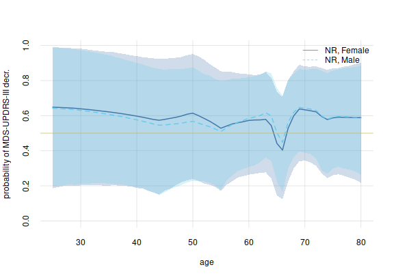
plot of chunk unnamed-chunk-28
(TO BE CONTINUED)