27 Inference about frequencies
\(\DeclarePairedDelimiter{\set}{\{}{\}}\) \(\DeclarePairedDelimiter{\abs}{\lvert}{\rvert}\)
27.1 Inference when population frequencies aren’t known
In chapter 26 we considered an agent that has exchangeable beliefs and that knows the full-population frequencies. The degrees of belief of such an agent have a very simple form: products of frequencies. But for such an agent the observations of units doesn’t give any useful information for drawing inferences about new units: such observations provide frequencies which the agent already knows.
Situations where we have complete frequency knowledge can be common in engineering problems, where the physical laws underlying the phenomena involved are known and computable. They are far less common in data-science and machine-learning applications: here we must consider agents that do not know the full-population frequencies.
How does such an agent calculate probabilities about units? The answer is actually a simple application of the “extension of the conversation” (§ 9.5, which boil down to applications of the and and or rules). A probability given that the frequency distribution is not known is equal to the average of the probabilities given each possible frequency distribution, weighted by the probabilities of the frequency distributions:
\[ \begin{aligned} &\mathrm{P}( Z_{u'}\mathclose{}\mathord{\nonscript\mkern 0mu\textrm{\small=}\nonscript\mkern 0mu}\mathopen{}{ z'} \mathbin{\mkern-0.5mu,\mkern-0.5mu} Z_{u''}\mathclose{}\mathord{\nonscript\mkern 0mu\textrm{\small=}\nonscript\mkern 0mu}\mathopen{}{ z''} \mathbin{\mkern-0.5mu,\mkern-0.5mu} \dotsb \nonscript\:\vert\nonscript\:\mathopen{} \mathsfit{I} ) \\[2ex] &\qquad{}= \sum_{\boldsymbol{f}} \mathrm{P}( Z_{u'}\mathclose{}\mathord{\nonscript\mkern 0mu\textrm{\small=}\nonscript\mkern 0mu}\mathopen{}{ z'} \mathbin{\mkern-0.5mu,\mkern-0.5mu} Z_{u''}\mathclose{}\mathord{\nonscript\mkern 0mu\textrm{\small=}\nonscript\mkern 0mu}\mathopen{}{ z''} \mathbin{\mkern-0.5mu,\mkern-0.5mu} \dotsb \nonscript\:\vert\nonscript\:\mathopen{} F\mathclose{}\mathord{\nonscript\mkern 0mu\textrm{\small=}\nonscript\mkern 0mu}\mathopen{}\boldsymbol{f}\mathbin{\mkern-0.5mu,\mkern-0.5mu}\mathsfit{I} ) \cdot \mathrm{P}(F\mathclose{}\mathord{\nonscript\mkern 0mu\textrm{\small=}\nonscript\mkern 0mu}\mathopen{}\boldsymbol{f}\nonscript\:\vert\nonscript\:\mathopen{} \mathsfit{I}) \end{aligned} \]
But we saw in § 26.4 that the probability for a sequence of values given a known frequency is just the product of the value’s frequencies. We thus have our long-sought formula:
This result is called de Finetti’s representation theorem for exchangeable belief distributions. It must be emphasized that this result is actually independent of any real or imaginary population frequencies. We took a route to it through the idea of population frequencies only to help our intuition. If for any reason you find the idea of a “limit frequency for an infinite population” somewhat suspicious, then don’t worry: the formula above actually does not rely on it. The formula results from the assumption has exchangeable beliefs about a collection of units that can potentially be continued without end.
Let’s see how this formula works in the simple Mars-prospecting example (with 3 million rocks or more) from § 26.4. Suppose that the agent:
knows that the rock collection consists of:
either a proportion 2/3 of \({\color[RGB]{102,204,238}{\small\verb;Y;}}\)-rocks and 1/3 of \({\color[RGB]{204,187,68}{\small\verb;N;}}\)-rocks; denote these frequencies with \(\boldsymbol{f}'\)
or a proportion 1/2 of \({\color[RGB]{102,204,238}{\small\verb;Y;}}\)-rocks and 1/2 of \({\color[RGB]{204,187,68}{\small\verb;N;}}\)-rocks; denote these frequencies with \(\boldsymbol{f}''\)
assigns a \(75\%\) degree of belief to the first hypothesis, and \(25\%\) to the second (so the sentence \((F\mathclose{}\mathord{\nonscript\mkern 0mu\textrm{\small=}\nonscript\mkern 0mu}\mathopen{}\boldsymbol{f}') \lor (F\mathclose{}\mathord{\nonscript\mkern 0mu\textrm{\small=}\nonscript\mkern 0mu}\mathopen{}\boldsymbol{f}'')\) has probability \(1\)):
\[ \mathrm{P}(F\mathclose{}\mathord{\nonscript\mkern 0mu\textrm{\small=}\nonscript\mkern 0mu}\mathopen{}\boldsymbol{f}'\nonscript\:\vert\nonscript\:\mathopen{} \mathsfit{K}) = 75\% \qquad \mathrm{P}(F\mathclose{}\mathord{\nonscript\mkern 0mu\textrm{\small=}\nonscript\mkern 0mu}\mathopen{}\boldsymbol{f}''\nonscript\:\vert\nonscript\:\mathopen{} \mathsfit{K}) = 25\% \]
What is the agent’s degree of belief that rock #1 contains haematite? According to the derived rule of extension of the conversation, that is, the main formula written above, we find:
\[ \begin{aligned} \mathrm{P}(R_{1} \mathclose{}\mathord{\nonscript\mkern 0mu\textrm{\small=}\nonscript\mkern 0mu}\mathopen{}{\color[RGB]{102,204,238}{\small\verb;Y;}}\nonscript\:\vert\nonscript\:\mathopen{} \mathsfit{K}) &= \sum_{\boldsymbol{f}} f(R\mathclose{}\mathord{\nonscript\mkern 0mu\textrm{\small=}\nonscript\mkern 0mu}\mathopen{}{\color[RGB]{102,204,238}{\small\verb;Y;}}) \cdot \mathrm{P}(F\mathclose{}\mathord{\nonscript\mkern 0mu\textrm{\small=}\nonscript\mkern 0mu}\mathopen{}\boldsymbol{f}\nonscript\:\vert\nonscript\:\mathopen{} \mathsfit{K}) \\[1ex] &= f'(R\mathclose{}\mathord{\nonscript\mkern 0mu\textrm{\small=}\nonscript\mkern 0mu}\mathopen{}{\color[RGB]{102,204,238}{\small\verb;Y;}}) \cdot \mathrm{P}(F\mathclose{}\mathord{\nonscript\mkern 0mu\textrm{\small=}\nonscript\mkern 0mu}\mathopen{}\boldsymbol{f}'\nonscript\:\vert\nonscript\:\mathopen{} \mathsfit{K}) + f''(R\mathclose{}\mathord{\nonscript\mkern 0mu\textrm{\small=}\nonscript\mkern 0mu}\mathopen{}{\color[RGB]{102,204,238}{\small\verb;Y;}}) \cdot \mathrm{P}(F\mathclose{}\mathord{\nonscript\mkern 0mu\textrm{\small=}\nonscript\mkern 0mu}\mathopen{}\boldsymbol{f}''\nonscript\:\vert\nonscript\:\mathopen{} \mathsfit{K}) \\[1ex] &= {\color[RGB]{102,204,238}\frac{2}{3}}\cdot 75\% + {\color[RGB]{102,204,238}\frac{1}{2}}\cdot 25\% \\[1ex] &= \boldsymbol{62.5\%} \end{aligned} \]
In an analogous way we can calculate, for instance, the agent’s belief that rock #1 contains haematite, rock #2 doesn’t, and rock #3 does:
\[ \begin{aligned} \mathrm{P}(R_{1} \mathclose{}\mathord{\nonscript\mkern 0mu\textrm{\small=}\nonscript\mkern 0mu}\mathopen{}{\color[RGB]{102,204,238}{\small\verb;Y;}}\mathbin{\mkern-0.5mu,\mkern-0.5mu}R_{2} \mathclose{}\mathord{\nonscript\mkern 0mu\textrm{\small=}\nonscript\mkern 0mu}\mathopen{}{\color[RGB]{204,187,68}{\small\verb;N;}}\mathbin{\mkern-0.5mu,\mkern-0.5mu}R_{3} \mathclose{}\mathord{\nonscript\mkern 0mu\textrm{\small=}\nonscript\mkern 0mu}\mathopen{}{\color[RGB]{102,204,238}{\small\verb;Y;}}\nonscript\:\vert\nonscript\:\mathopen{} \mathsfit{K}) &\approx \sum_{\boldsymbol{f}} f(R\mathclose{}\mathord{\nonscript\mkern 0mu\textrm{\small=}\nonscript\mkern 0mu}\mathopen{}{\color[RGB]{102,204,238}{\small\verb;Y;}}) \cdot f(R\mathclose{}\mathord{\nonscript\mkern 0mu\textrm{\small=}\nonscript\mkern 0mu}\mathopen{}{\color[RGB]{204,187,68}{\small\verb;N;}}) \cdot f(R\mathclose{}\mathord{\nonscript\mkern 0mu\textrm{\small=}\nonscript\mkern 0mu}\mathopen{}{\color[RGB]{102,204,238}{\small\verb;Y;}}) \cdot \mathrm{P}(F\mathclose{}\mathord{\nonscript\mkern 0mu\textrm{\small=}\nonscript\mkern 0mu}\mathopen{}\boldsymbol{f}\nonscript\:\vert\nonscript\:\mathopen{} \mathsfit{K}) \\[2ex] &= f'(R\mathclose{}\mathord{\nonscript\mkern 0mu\textrm{\small=}\nonscript\mkern 0mu}\mathopen{}{\color[RGB]{102,204,238}{\small\verb;Y;}}) \cdot f'(R\mathclose{}\mathord{\nonscript\mkern 0mu\textrm{\small=}\nonscript\mkern 0mu}\mathopen{}{\color[RGB]{204,187,68}{\small\verb;N;}}) \cdot f'(R\mathclose{}\mathord{\nonscript\mkern 0mu\textrm{\small=}\nonscript\mkern 0mu}\mathopen{}{\color[RGB]{102,204,238}{\small\verb;Y;}}) \cdot \mathrm{P}(F\mathclose{}\mathord{\nonscript\mkern 0mu\textrm{\small=}\nonscript\mkern 0mu}\mathopen{}\boldsymbol{f}'\nonscript\:\vert\nonscript\:\mathopen{} \mathsfit{K}) + {} \\[1ex] &\qquad f''(R\mathclose{}\mathord{\nonscript\mkern 0mu\textrm{\small=}\nonscript\mkern 0mu}\mathopen{}{\color[RGB]{102,204,238}{\small\verb;Y;}}) \cdot f''(R\mathclose{}\mathord{\nonscript\mkern 0mu\textrm{\small=}\nonscript\mkern 0mu}\mathopen{}{\color[RGB]{204,187,68}{\small\verb;N;}}) \cdot f''(R\mathclose{}\mathord{\nonscript\mkern 0mu\textrm{\small=}\nonscript\mkern 0mu}\mathopen{}{\color[RGB]{102,204,238}{\small\verb;Y;}}) \cdot \mathrm{P}(F\mathclose{}\mathord{\nonscript\mkern 0mu\textrm{\small=}\nonscript\mkern 0mu}\mathopen{}\boldsymbol{f}''\nonscript\:\vert\nonscript\:\mathopen{} \mathsfit{K}) \\[2ex] &= {\color[RGB]{102,204,238}\frac{2}{3}}\cdot {\color[RGB]{204,187,68}\frac{1}{3}}\cdot {\color[RGB]{102,204,238}\frac{2}{3}}\cdot 75\% + {\color[RGB]{102,204,238}\frac{1}{2}}\cdot {\color[RGB]{204,187,68}\frac{1}{2}}\cdot {\color[RGB]{102,204,238}\frac{1}{2}}\cdot 25\% \\[2ex] &\approx \boldsymbol{14.236\%} \end{aligned} \]
This formula generalizes to any population, any variates, and any number of hypotheses about the frequencies.
Mathematical and, even more, computational complications arise when we consider all possible frequency distributions, since there is a practically infinite number of them; they form a continuum in fact. But do not let these practical difficulties affect the intuitive picture behind them, which is simple to grasp once you’ve considered some simple examples.
Consider a state of knowledge \(\mathsfit{K}'\) according to which:
- The rock collection may have a proportion \(0/10\) of \({\color[RGB]{102,204,238}{\small\verb;Y;}}\)-rocks (and \(10/10\) of \({\color[RGB]{204,187,68}{\small\verb;N;}}\)-rocks); call this frequency distribution \(\boldsymbol{f}_0\)
- The rock collection may have a proportion \(1/10\) of \({\color[RGB]{102,204,238}{\small\verb;Y;}}\)-rocks; call this \(\boldsymbol{f}_1\)
- and so on… up to
- a proportion \(10/10\) of \({\color[RGB]{102,204,238}{\small\verb;Y;}}\)-rocks; call this \(\boldsymbol{f}_{10}\)
The probability of each of these frequency hypotheses is \(1/11\), that is:
\[ \begin{aligned} &\mathrm{P}(F\mathclose{}\mathord{\nonscript\mkern 0mu\textrm{\small=}\nonscript\mkern 0mu}\mathopen{}\boldsymbol{f}_{0} \nonscript\:\vert\nonscript\:\mathopen{} \mathsfit{K}') = 1/11 \\[1ex] &\mathrm{P}(F\mathclose{}\mathord{\nonscript\mkern 0mu\textrm{\small=}\nonscript\mkern 0mu}\mathopen{}\boldsymbol{f}_{1} \nonscript\:\vert\nonscript\:\mathopen{} \mathsfit{K}') = 1/11 \\[1ex] &\dotso\\[1ex] &\mathrm{P}(F\mathclose{}\mathord{\nonscript\mkern 0mu\textrm{\small=}\nonscript\mkern 0mu}\mathopen{}\boldsymbol{f}_{10} \nonscript\:\vert\nonscript\:\mathopen{} \mathsfit{K}') = 1/11 \end{aligned} \]
Calculate the probabilities
\[ \mathrm{P}(R_1\mathclose{}\mathord{\nonscript\mkern 0mu\textrm{\small=}\nonscript\mkern 0mu}\mathopen{}{\color[RGB]{102,204,238}{\small\verb;Y;}}\mathbin{\mkern-0.5mu,\mkern-0.5mu}R_2\mathclose{}\mathord{\nonscript\mkern 0mu\textrm{\small=}\nonscript\mkern 0mu}\mathopen{}{\color[RGB]{102,204,238}{\small\verb;Y;}}\nonscript\:\vert\nonscript\:\mathopen{}\mathsfit{K}') \qquad \mathrm{P}(R_1\mathclose{}\mathord{\nonscript\mkern 0mu\textrm{\small=}\nonscript\mkern 0mu}\mathopen{}{\color[RGB]{102,204,238}{\small\verb;Y;}}\mathbin{\mkern-0.5mu,\mkern-0.5mu}R_2\mathclose{}\mathord{\nonscript\mkern 0mu\textrm{\small=}\nonscript\mkern 0mu}\mathopen{}{\color[RGB]{204,187,68}{\small\verb;N;}}\nonscript\:\vert\nonscript\:\mathopen{}\mathsfit{K}') \qquad \mathrm{P}(R_1\mathclose{}\mathord{\nonscript\mkern 0mu\textrm{\small=}\nonscript\mkern 0mu}\mathopen{}{\color[RGB]{204,187,68}{\small\verb;N;}}\mathbin{\mkern-0.5mu,\mkern-0.5mu}R_2\mathclose{}\mathord{\nonscript\mkern 0mu\textrm{\small=}\nonscript\mkern 0mu}\mathopen{}{\color[RGB]{204,187,68}{\small\verb;N;}}\nonscript\:\vert\nonscript\:\mathopen{}\mathsfit{K}') \]
Do they all have the same value? Try to explain why or why not.
27.2 Learning from observed units
Staying with the same Mars-prospecting scenario, let’s now ask what’s the agent’s degree of belief that rock #1 contains haematite, given that the agent has found that rock #2 doesn’t contain haematite. In the case of an agent that knows the full-population frequencies we saw § 26.5 that this degree of belief is actually unaffected by other observations. What happens when the population frequencies are not known?
The calculation is straightforward:
\[ \begin{aligned} \mathrm{P}(R_{1} \mathclose{}\mathord{\nonscript\mkern 0mu\textrm{\small=}\nonscript\mkern 0mu}\mathopen{}{\color[RGB]{102,204,238}{\small\verb;Y;}}\nonscript\:\vert\nonscript\:\mathopen{} R_{2} \mathclose{}\mathord{\nonscript\mkern 0mu\textrm{\small=}\nonscript\mkern 0mu}\mathopen{}{\color[RGB]{204,187,68}{\small\verb;N;}}\mathbin{\mkern-0.5mu,\mkern-0.5mu}\mathsfit{K}) &= \frac{ \mathrm{P}(R_{1} \mathclose{}\mathord{\nonscript\mkern 0mu\textrm{\small=}\nonscript\mkern 0mu}\mathopen{}{\color[RGB]{102,204,238}{\small\verb;Y;}}\mathbin{\mkern-0.5mu,\mkern-0.5mu}R_{2} \mathclose{}\mathord{\nonscript\mkern 0mu\textrm{\small=}\nonscript\mkern 0mu}\mathopen{}{\color[RGB]{204,187,68}{\small\verb;N;}}\nonscript\:\vert\nonscript\:\mathopen{} \mathsfit{K}) }{ \mathrm{P}(R_{2} \mathclose{}\mathord{\nonscript\mkern 0mu\textrm{\small=}\nonscript\mkern 0mu}\mathopen{}{\color[RGB]{204,187,68}{\small\verb;N;}}\nonscript\:\vert\nonscript\:\mathopen{} \mathsfit{K}) } \\[2ex] &\approx \frac{ \sum_{\boldsymbol{f}} f(R\mathclose{}\mathord{\nonscript\mkern 0mu\textrm{\small=}\nonscript\mkern 0mu}\mathopen{}{\color[RGB]{102,204,238}{\small\verb;Y;}}) \cdot f(R\mathclose{}\mathord{\nonscript\mkern 0mu\textrm{\small=}\nonscript\mkern 0mu}\mathopen{}{\color[RGB]{204,187,68}{\small\verb;N;}}) \cdot \mathrm{P}(F\mathclose{}\mathord{\nonscript\mkern 0mu\textrm{\small=}\nonscript\mkern 0mu}\mathopen{}\boldsymbol{f}\nonscript\:\vert\nonscript\:\mathopen{} \mathsfit{K}) }{ \sum_{\boldsymbol{f}} f(R\mathclose{}\mathord{\nonscript\mkern 0mu\textrm{\small=}\nonscript\mkern 0mu}\mathopen{}{\color[RGB]{204,187,68}{\small\verb;N;}}) \cdot \mathrm{P}(F\mathclose{}\mathord{\nonscript\mkern 0mu\textrm{\small=}\nonscript\mkern 0mu}\mathopen{}\boldsymbol{f}\nonscript\:\vert\nonscript\:\mathopen{} \mathsfit{K}) } \\[2ex] &= \frac{ {\color[RGB]{102,204,238}\frac{2}{3}}\cdot {\color[RGB]{204,187,68}\frac{1}{3}}\cdot 75\% + {\color[RGB]{102,204,238}\frac{1}{2}}\cdot {\color[RGB]{204,187,68}\frac{1}{2}}\cdot 25\% }{ {\color[RGB]{204,187,68}\frac{1}{3}}\cdot 75\% + {\color[RGB]{204,187,68}\frac{1}{2}}\cdot 25\% } \\[2ex] &\approx\frac{ 22.9167\% }{ 37.5000\% } \\[2ex] &= \boldsymbol{61.111\%} \end{aligned} \]
Knowledge that \(R_{2}\mathclose{}\mathord{\nonscript\mkern 0mu\textrm{\small=}\nonscript\mkern 0mu}\mathopen{}{\color[RGB]{204,187,68}{\small\verb;N;}}\) thus does affect the agent’s belief about \(R_{1}\mathclose{}\mathord{\nonscript\mkern 0mu\textrm{\small=}\nonscript\mkern 0mu}\mathopen{}{\color[RGB]{102,204,238}{\small\verb;Y;}}\):
\[ \mathrm{P}(R_{1} \mathclose{}\mathord{\nonscript\mkern 0mu\textrm{\small=}\nonscript\mkern 0mu}\mathopen{}{\color[RGB]{102,204,238}{\small\verb;Y;}}\nonscript\:\vert\nonscript\:\mathopen{} \mathsfit{K}) = 62.5\% \qquad \mathrm{P}(R_{1} \mathclose{}\mathord{\nonscript\mkern 0mu\textrm{\small=}\nonscript\mkern 0mu}\mathopen{}{\color[RGB]{102,204,238}{\small\verb;Y;}}\nonscript\:\vert\nonscript\:\mathopen{} R_{2} \mathclose{}\mathord{\nonscript\mkern 0mu\textrm{\small=}\nonscript\mkern 0mu}\mathopen{}{\color[RGB]{204,187,68}{\small\verb;N;}}\mathbin{\mkern-0.5mu,\mkern-0.5mu}\mathsfit{K}) \approx 61.1\% \]
In particular, the observation of one \({\color[RGB]{204,187,68}{\small\verb;N;}}\)-rock has somewhat decreased the probability of observing a new \({\color[RGB]{102,204,238}{\small\verb;Y;}}\)-rock.
Calculate the minimal number of \({\color[RGB]{204,187,68}{\small\verb;N;}}\) observations needed for lowering the agent’s degree of belief of observing a \({\color[RGB]{102,204,238}{\small\verb;Y;}}\) to \(55\%\) or less.
Does it seem possible to lower the agent’s belief to less than \(50\%\)? Explain why.
Calculate the minimal number of \({\color[RGB]{102,204,238}{\small\verb;Y;}}\) observations needed for increasing the agent’s degree of belief of observing a \({\color[RGB]{102,204,238}{\small\verb;Y;}}\) to \(65\%\) or more.
Does it seem possible to increase the agent’s belief to more than \(2/3\)? Explain why.
27.3 How learning works: learning about frequencies
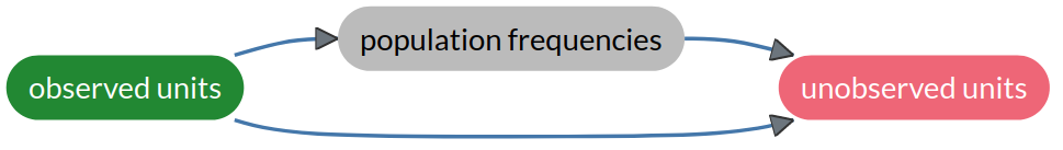
An agent having full-population frequency information does not learn1 from observation of units, whereas an agent not having such information does learn from observation of units. This fact shows how learning from observed to unobserved units actually works. Crudely speaking, observations do not directly affect the beliefs about unobserved units, but instead affect the beliefs about the population frequencies. And these in turn affect the beliefs about unobserved units. Graphically this could be represented as follows:
1 remember the warning of § 26.5 about “learning”

as opposed to this:
The informational relation between observed units, frequencies, and unobserved units becomes clear if we check how the agent’s beliefs about the frequency hypotheses change as observations are made. In the Mars-prospecting example of § 27.1, the agent has initial probabilities
\[ \mathrm{P}(F\mathclose{}\mathord{\nonscript\mkern 0mu\textrm{\small=}\nonscript\mkern 0mu}\mathopen{}\boldsymbol{f}'\nonscript\:\vert\nonscript\:\mathopen{} \mathsfit{K}) = 75\% \qquad \mathrm{P}(F\mathclose{}\mathord{\nonscript\mkern 0mu\textrm{\small=}\nonscript\mkern 0mu}\mathopen{}\boldsymbol{f}''\nonscript\:\vert\nonscript\:\mathopen{} \mathsfit{K}) = 25\% \]
where \(\boldsymbol{f}'\) gives frequency \(2/3\) to \({\color[RGB]{102,204,238}{\small\verb;Y;}}\), and \(\boldsymbol{f}''\) gives frequency \(1/2\) to \({\color[RGB]{102,204,238}{\small\verb;Y;}}\). How do these probabilities change, conditional on the agent’s observing that rock #2 doesn’t contain haematite? We just need to use Bayes’s theorem. For the first hypothesis \(F\mathclose{}\mathord{\nonscript\mkern 0mu\textrm{\small=}\nonscript\mkern 0mu}\mathopen{}\boldsymbol{f}'\):
\[ \begin{aligned} \mathrm{P}(F\mathclose{}\mathord{\nonscript\mkern 0mu\textrm{\small=}\nonscript\mkern 0mu}\mathopen{}\boldsymbol{f}'\nonscript\:\vert\nonscript\:\mathopen{} R_2\mathclose{}\mathord{\nonscript\mkern 0mu\textrm{\small=}\nonscript\mkern 0mu}\mathopen{}{\color[RGB]{204,187,68}{\small\verb;N;}}\mathbin{\mkern-0.5mu,\mkern-0.5mu}\mathsfit{K}) &= \frac{ \mathrm{P}(R_2\mathclose{}\mathord{\nonscript\mkern 0mu\textrm{\small=}\nonscript\mkern 0mu}\mathopen{}{\color[RGB]{204,187,68}{\small\verb;N;}}\nonscript\:\vert\nonscript\:\mathopen{} F\mathclose{}\mathord{\nonscript\mkern 0mu\textrm{\small=}\nonscript\mkern 0mu}\mathopen{}\boldsymbol{f}'\mathbin{\mkern-0.5mu,\mkern-0.5mu}\mathsfit{K}) \cdot \mathrm{P}(F\mathclose{}\mathord{\nonscript\mkern 0mu\textrm{\small=}\nonscript\mkern 0mu}\mathopen{}\boldsymbol{f}'\nonscript\:\vert\nonscript\:\mathopen{} \mathsfit{K}) }{ \mathrm{P}(R_2\mathclose{}\mathord{\nonscript\mkern 0mu\textrm{\small=}\nonscript\mkern 0mu}\mathopen{}{\color[RGB]{204,187,68}{\small\verb;N;}}\nonscript\:\vert\nonscript\:\mathopen{} F\mathclose{}\mathord{\nonscript\mkern 0mu\textrm{\small=}\nonscript\mkern 0mu}\mathopen{}\boldsymbol{f}'\mathbin{\mkern-0.5mu,\mkern-0.5mu}\mathsfit{K}) \cdot \mathrm{P}(F\mathclose{}\mathord{\nonscript\mkern 0mu\textrm{\small=}\nonscript\mkern 0mu}\mathopen{}\boldsymbol{f}'\nonscript\:\vert\nonscript\:\mathopen{} \mathsfit{K}) + \mathrm{P}(R_2\mathclose{}\mathord{\nonscript\mkern 0mu\textrm{\small=}\nonscript\mkern 0mu}\mathopen{}{\color[RGB]{204,187,68}{\small\verb;N;}}\nonscript\:\vert\nonscript\:\mathopen{} F\mathclose{}\mathord{\nonscript\mkern 0mu\textrm{\small=}\nonscript\mkern 0mu}\mathopen{}\boldsymbol{f}''\mathbin{\mkern-0.5mu,\mkern-0.5mu}\mathsfit{K}) \cdot \mathrm{P}(F\mathclose{}\mathord{\nonscript\mkern 0mu\textrm{\small=}\nonscript\mkern 0mu}\mathopen{}\boldsymbol{f}''\nonscript\:\vert\nonscript\:\mathopen{} \mathsfit{K}) } \\[1ex] &= \frac{ f'(R\mathclose{}\mathord{\nonscript\mkern 0mu\textrm{\small=}\nonscript\mkern 0mu}\mathopen{}{\color[RGB]{204,187,68}{\small\verb;N;}}) \cdot \mathrm{P}(F\mathclose{}\mathord{\nonscript\mkern 0mu\textrm{\small=}\nonscript\mkern 0mu}\mathopen{}\boldsymbol{f}'\nonscript\:\vert\nonscript\:\mathopen{} \mathsfit{K}) }{ f'(R\mathclose{}\mathord{\nonscript\mkern 0mu\textrm{\small=}\nonscript\mkern 0mu}\mathopen{}{\color[RGB]{204,187,68}{\small\verb;N;}}) \cdot \mathrm{P}(F\mathclose{}\mathord{\nonscript\mkern 0mu\textrm{\small=}\nonscript\mkern 0mu}\mathopen{}\boldsymbol{f}'\nonscript\:\vert\nonscript\:\mathopen{} \mathsfit{K}) + f''(R\mathclose{}\mathord{\nonscript\mkern 0mu\textrm{\small=}\nonscript\mkern 0mu}\mathopen{}{\color[RGB]{204,187,68}{\small\verb;N;}}) \cdot \mathrm{P}(F\mathclose{}\mathord{\nonscript\mkern 0mu\textrm{\small=}\nonscript\mkern 0mu}\mathopen{}\boldsymbol{f}''\nonscript\:\vert\nonscript\:\mathopen{} \mathsfit{K}) } \\[1ex] &= \frac{ \frac{1}{3} \cdot 75\% }{ \frac{1}{3} \cdot 75\% + \frac{1}{2} \cdot 25\% } \\[2ex] &= \boldsymbol{66.667\%} \end{aligned} \]
and an analogous calculation yields \(\mathrm{P}(F\mathclose{}\mathord{\nonscript\mkern 0mu\textrm{\small=}\nonscript\mkern 0mu}\mathopen{}\boldsymbol{f}''\nonscript\:\vert\nonscript\:\mathopen{} R_2\mathclose{}\mathord{\nonscript\mkern 0mu\textrm{\small=}\nonscript\mkern 0mu}\mathopen{}{\color[RGB]{204,187,68}{\small\verb;N;}}\mathbin{\mkern-0.5mu,\mkern-0.5mu}\mathsfit{K})=33.333\%\).
This result makes sense, because according to the hypothesis \(F\mathclose{}\mathord{\nonscript\mkern 0mu\textrm{\small=}\nonscript\mkern 0mu}\mathopen{}\boldsymbol{f}''\) there is a higher proportion of \({\color[RGB]{204,187,68}{\small\verb;N;}}\)-rocks than according to \(F\mathclose{}\mathord{\nonscript\mkern 0mu\textrm{\small=}\nonscript\mkern 0mu}\mathopen{}\boldsymbol{f}'\), and a \({\color[RGB]{204,187,68}{\small\verb;N;}}\)-rock has been observed. The hypothesis \(F\mathclose{}\mathord{\nonscript\mkern 0mu\textrm{\small=}\nonscript\mkern 0mu}\mathopen{}\boldsymbol{f}''\) therefore becomes slightly more plausible, and \(F\mathclose{}\mathord{\nonscript\mkern 0mu\textrm{\small=}\nonscript\mkern 0mu}\mathopen{}\boldsymbol{f}'\) slightly less.
The updated degree of belief above for the frequencies also gives us an alternative (yet equivalent) way to calculate the conditional probability \(\mathrm{P}(R_{1} \mathclose{}\mathord{\nonscript\mkern 0mu\textrm{\small=}\nonscript\mkern 0mu}\mathopen{}{\color[RGB]{102,204,238}{\small\verb;Y;}}\nonscript\:\vert\nonscript\:\mathopen{} R_{2} \mathclose{}\mathord{\nonscript\mkern 0mu\textrm{\small=}\nonscript\mkern 0mu}\mathopen{}{\color[RGB]{204,187,68}{\small\verb;N;}}\mathbin{\mkern-0.5mu,\mkern-0.5mu}\mathsfit{K})\). Use the derived rule of “extension of the conversation” in a different manner:
\[ \begin{aligned} \mathrm{P}(R_{1} \mathclose{}\mathord{\nonscript\mkern 0mu\textrm{\small=}\nonscript\mkern 0mu}\mathopen{}{\color[RGB]{102,204,238}{\small\verb;Y;}}\nonscript\:\vert\nonscript\:\mathopen{} R_{2} \mathclose{}\mathord{\nonscript\mkern 0mu\textrm{\small=}\nonscript\mkern 0mu}\mathopen{}{\color[RGB]{204,187,68}{\small\verb;N;}}\mathbin{\mkern-0.5mu,\mkern-0.5mu}\mathsfit{K}) &= \sum_{\boldsymbol{f}} \mathrm{P}(R_{1} \mathclose{}\mathord{\nonscript\mkern 0mu\textrm{\small=}\nonscript\mkern 0mu}\mathopen{}{\color[RGB]{102,204,238}{\small\verb;Y;}}\nonscript\:\vert\nonscript\:\mathopen{} R_{2} \mathclose{}\mathord{\nonscript\mkern 0mu\textrm{\small=}\nonscript\mkern 0mu}\mathopen{}{\color[RGB]{204,187,68}{\small\verb;N;}}\mathbin{\mkern-0.5mu,\mkern-0.5mu}F\mathclose{}\mathord{\nonscript\mkern 0mu\textrm{\small=}\nonscript\mkern 0mu}\mathopen{}\boldsymbol{f}\mathbin{\mkern-0.5mu,\mkern-0.5mu}\mathsfit{K}) \cdot \mathrm{P}(F\mathclose{}\mathord{\nonscript\mkern 0mu\textrm{\small=}\nonscript\mkern 0mu}\mathopen{}\boldsymbol{f}\nonscript\:\vert\nonscript\:\mathopen{} R_{2} \mathclose{}\mathord{\nonscript\mkern 0mu\textrm{\small=}\nonscript\mkern 0mu}\mathopen{}{\color[RGB]{204,187,68}{\small\verb;N;}}\mathbin{\mkern-0.5mu,\mkern-0.5mu}\mathsfit{K}) \\[2ex] \text{\color[RGB]{187,187,187}\scriptsize(no learning if frequencies are known)}\enspace &=\sum_{\boldsymbol{f}} \mathrm{P}(R_{1} \mathclose{}\mathord{\nonscript\mkern 0mu\textrm{\small=}\nonscript\mkern 0mu}\mathopen{}{\color[RGB]{102,204,238}{\small\verb;Y;}}\nonscript\:\vert\nonscript\:\mathopen{} F\mathclose{}\mathord{\nonscript\mkern 0mu\textrm{\small=}\nonscript\mkern 0mu}\mathopen{}\boldsymbol{f}\mathbin{\mkern-0.5mu,\mkern-0.5mu}\mathsfit{K}) \cdot \mathrm{P}(F\mathclose{}\mathord{\nonscript\mkern 0mu\textrm{\small=}\nonscript\mkern 0mu}\mathopen{}\boldsymbol{f}\nonscript\:\vert\nonscript\:\mathopen{} R_{2} \mathclose{}\mathord{\nonscript\mkern 0mu\textrm{\small=}\nonscript\mkern 0mu}\mathopen{}{\color[RGB]{204,187,68}{\small\verb;N;}}\mathbin{\mkern-0.5mu,\mkern-0.5mu}\mathsfit{K}) \\[2ex] &= \mathrm{P}(R_{1} \mathclose{}\mathord{\nonscript\mkern 0mu\textrm{\small=}\nonscript\mkern 0mu}\mathopen{}{\color[RGB]{102,204,238}{\small\verb;Y;}}\nonscript\:\vert\nonscript\:\mathopen{} F\mathclose{}\mathord{\nonscript\mkern 0mu\textrm{\small=}\nonscript\mkern 0mu}\mathopen{}\boldsymbol{f}'\mathbin{\mkern-0.5mu,\mkern-0.5mu}\mathsfit{K}) \cdot \mathrm{P}(F\mathclose{}\mathord{\nonscript\mkern 0mu\textrm{\small=}\nonscript\mkern 0mu}\mathopen{}\boldsymbol{f}'\nonscript\:\vert\nonscript\:\mathopen{} R_{2} \mathclose{}\mathord{\nonscript\mkern 0mu\textrm{\small=}\nonscript\mkern 0mu}\mathopen{}{\color[RGB]{204,187,68}{\small\verb;N;}}\mathbin{\mkern-0.5mu,\mkern-0.5mu}\mathsfit{K}) +{} \\[1ex] &\qquad\mathrm{P}(R_{1} \mathclose{}\mathord{\nonscript\mkern 0mu\textrm{\small=}\nonscript\mkern 0mu}\mathopen{}{\color[RGB]{102,204,238}{\small\verb;Y;}}\nonscript\:\vert\nonscript\:\mathopen{} F\mathclose{}\mathord{\nonscript\mkern 0mu\textrm{\small=}\nonscript\mkern 0mu}\mathopen{}\boldsymbol{f}''\mathbin{\mkern-0.5mu,\mkern-0.5mu}\mathsfit{K}) \cdot \mathrm{P}(F\mathclose{}\mathord{\nonscript\mkern 0mu\textrm{\small=}\nonscript\mkern 0mu}\mathopen{}\boldsymbol{f}''\nonscript\:\vert\nonscript\:\mathopen{} R_{2} \mathclose{}\mathord{\nonscript\mkern 0mu\textrm{\small=}\nonscript\mkern 0mu}\mathopen{}{\color[RGB]{204,187,68}{\small\verb;N;}}\mathbin{\mkern-0.5mu,\mkern-0.5mu}\mathsfit{K}) \\[2ex] &= f'(R\mathclose{}\mathord{\nonscript\mkern 0mu\textrm{\small=}\nonscript\mkern 0mu}\mathopen{}{\color[RGB]{102,204,238}{\small\verb;Y;}}) \cdot \mathrm{P}(F\mathclose{}\mathord{\nonscript\mkern 0mu\textrm{\small=}\nonscript\mkern 0mu}\mathopen{}\boldsymbol{f}'\nonscript\:\vert\nonscript\:\mathopen{} R_{2} \mathclose{}\mathord{\nonscript\mkern 0mu\textrm{\small=}\nonscript\mkern 0mu}\mathopen{}{\color[RGB]{204,187,68}{\small\verb;N;}}\mathbin{\mkern-0.5mu,\mkern-0.5mu}\mathsfit{K}) +{} \\[1ex] &\qquad f''(R\mathclose{}\mathord{\nonscript\mkern 0mu\textrm{\small=}\nonscript\mkern 0mu}\mathopen{}{\color[RGB]{102,204,238}{\small\verb;Y;}}) \cdot \mathrm{P}(F\mathclose{}\mathord{\nonscript\mkern 0mu\textrm{\small=}\nonscript\mkern 0mu}\mathopen{}\boldsymbol{f}''\nonscript\:\vert\nonscript\:\mathopen{} R_{2} \mathclose{}\mathord{\nonscript\mkern 0mu\textrm{\small=}\nonscript\mkern 0mu}\mathopen{}{\color[RGB]{204,187,68}{\small\verb;N;}}\mathbin{\mkern-0.5mu,\mkern-0.5mu}\mathsfit{K}) \\[2ex] &= {\color[RGB]{102,204,238}\frac{2}{3}} \cdot 66.667\% + {\color[RGB]{102,204,238}\frac{1}{2}} \cdot 33.333\% \\[2ex] &= \boldsymbol{61.111\%} \end{aligned} \]
The result is exactly as in § 27.2 – as it should be: remember from chapter 8 that the four rules of inference are built so as to mathematically guarantee this kind of logical self-consistency.
An intuitive interpretation of population inference
The general expression for the updated belief about frequencies has a very intuitive interpretation. Again using Bayes’s theorem, but omitting the proportionality constant,
\[ \begin{aligned} \mathrm{P}(F\mathclose{}\mathord{\nonscript\mkern 0mu\textrm{\small=}\nonscript\mkern 0mu}\mathopen{}\boldsymbol{f}\nonscript\:\vert\nonscript\:\mathopen{} \color[RGB]{34,136,51}Z_1\mathclose{}\mathord{\nonscript\mkern 0mu\textrm{\small=}\nonscript\mkern 0mu}\mathopen{}z_1 \mathbin{\mkern-0.5mu,\mkern-0.5mu}\dotsb \mathbin{\mkern-0.5mu,\mkern-0.5mu}Z_N\mathclose{}\mathord{\nonscript\mkern 0mu\textrm{\small=}\nonscript\mkern 0mu}\mathopen{}z_N \color[RGB]{0,0,0}\mathbin{\mkern-0.5mu,\mkern-0.5mu}\mathsfit{K}) &\propto \mathrm{P}(\color[RGB]{34,136,51}Z_1\mathclose{}\mathord{\nonscript\mkern 0mu\textrm{\small=}\nonscript\mkern 0mu}\mathopen{}z_1 \mathbin{\mkern-0.5mu,\mkern-0.5mu}\dotsb \mathbin{\mkern-0.5mu,\mkern-0.5mu}Z_N\mathclose{}\mathord{\nonscript\mkern 0mu\textrm{\small=}\nonscript\mkern 0mu}\mathopen{}z_N \color[RGB]{0,0,0} \nonscript\:\vert\nonscript\:\mathopen{} F\mathclose{}\mathord{\nonscript\mkern 0mu\textrm{\small=}\nonscript\mkern 0mu}\mathopen{}\boldsymbol{f}\mathbin{\mkern-0.5mu,\mkern-0.5mu}\mathsfit{K}) \cdot \mathrm{P}(F\mathclose{}\mathord{\nonscript\mkern 0mu\textrm{\small=}\nonscript\mkern 0mu}\mathopen{}\boldsymbol{f}\nonscript\:\vert\nonscript\:\mathopen{} \mathsfit{K}) \\[2ex] &\propto \overbracket[0.1ex]{f(\color[RGB]{34,136,51}Z_1\mathclose{}\mathord{\nonscript\mkern 0mu\textrm{\small=}\nonscript\mkern 0mu}\mathopen{}z_1\color[RGB]{0,0,0}) \cdot \,\dotsb\, \cdot f(\color[RGB]{34,136,51}Z_N\mathclose{}\mathord{\nonscript\mkern 0mu\textrm{\small=}\nonscript\mkern 0mu}\mathopen{}z_N \color[RGB]{0,0,0})}^{\color[RGB]{119,119,119}\mathclap{\text{how well the frequency "fits" the data}}} \ \cdot \ \underbracket[0.1ex]{\mathrm{P}(F\mathclose{}\mathord{\nonscript\mkern 0mu\textrm{\small=}\nonscript\mkern 0mu}\mathopen{}\boldsymbol{f}\nonscript\:\vert\nonscript\:\mathopen{} \mathsfit{K})}_{\color[RGB]{119,119,119}\mathclap{\text{how reasonable the frequency is}}} \end{aligned} \]
This product can be interpreted as follows.
Take a hypothetical frequency distribution \(\boldsymbol{f}\). If the data have high frequencies according to it, then the product
\[f(\color[RGB]{34,136,51}Z_1\mathclose{}\mathord{\nonscript\mkern 0mu\textrm{\small=}\nonscript\mkern 0mu}\mathopen{}z_1\color[RGB]{0,0,0}) \cdot \,\dotsb\, \cdot f(\color[RGB]{34,136,51}Z_N\mathclose{}\mathord{\nonscript\mkern 0mu\textrm{\small=}\nonscript\mkern 0mu}\mathopen{}z_N \color[RGB]{0,0,0})\]
has a large value. Vice versa, if the data have low frequency according to it, that product has a small value. This product therefore expresses how well the hypothetical frequency distribution \(\boldsymbol{f}\) “fits” the observed data.
On the other hand, if the factor
\[\mathrm{P}(F\mathclose{}\mathord{\nonscript\mkern 0mu\textrm{\small=}\nonscript\mkern 0mu}\mathopen{}\boldsymbol{f}\nonscript\:\vert\nonscript\:\mathopen{} \mathsfit{K})\]
has a large value, then the hypothetical \(\boldsymbol{f}\) is probable, or “reasonable”, according to the background information \(\mathsfit{K}\). Vice versa, if that factor has a low value, then the hypothetical \(\boldsymbol{f}\) is improbable or “unreasonable”, owing to reasons expressed in the background information \(\mathsfit{K}\).
The agent’s belief in the hypothetical \(\boldsymbol{f}\) is a balance between these two factors, the “fit” and the “reasonableness”. This has a very important consequence:
The agent’s belief about new data is then an average of what the frequency of the new data would be for all possible frequency distributions \(\boldsymbol{f}\):
\[ \begin{aligned} &\mathrm{P}(\color[RGB]{238,102,119}Z_{N+1}\mathclose{}\mathord{\nonscript\mkern 0mu\textrm{\small=}\nonscript\mkern 0mu}\mathopen{}z_{N+1} \color[RGB]{0,0,0}\nonscript\:\vert\nonscript\:\mathopen{} \color[RGB]{34,136,51}Z_1\mathclose{}\mathord{\nonscript\mkern 0mu\textrm{\small=}\nonscript\mkern 0mu}\mathopen{}z_1 \mathbin{\mkern-0.5mu,\mkern-0.5mu}\dotsb \mathbin{\mkern-0.5mu,\mkern-0.5mu}Z_N\mathclose{}\mathord{\nonscript\mkern 0mu\textrm{\small=}\nonscript\mkern 0mu}\mathopen{}z_N \color[RGB]{0,0,0}\mathbin{\mkern-0.5mu,\mkern-0.5mu}\mathsfit{K}) \\[2ex] &\qquad{}= \sum_{\boldsymbol{f}} f({\color[RGB]{238,102,119}Z_{N+1}\mathclose{}\mathord{\nonscript\mkern 0mu\textrm{\small=}\nonscript\mkern 0mu}\mathopen{}z_{N+1}}) \cdot \mathrm{P}(F\mathclose{}\mathord{\nonscript\mkern 0mu\textrm{\small=}\nonscript\mkern 0mu}\mathopen{}\boldsymbol{f}\nonscript\:\vert\nonscript\:\mathopen{} \color[RGB]{34,136,51}Z_1\mathclose{}\mathord{\nonscript\mkern 0mu\textrm{\small=}\nonscript\mkern 0mu}\mathopen{}z_1 \mathbin{\mkern-0.5mu,\mkern-0.5mu}\dotsb \mathbin{\mkern-0.5mu,\mkern-0.5mu}Z_N\mathclose{}\mathord{\nonscript\mkern 0mu\textrm{\small=}\nonscript\mkern 0mu}\mathopen{}z_N \color[RGB]{0,0,0}\mathbin{\mkern-0.5mu,\mkern-0.5mu}\mathsfit{K}) \end{aligned} \]
Each possible \(\boldsymbol{f}\) is weighed by its credibility, which takes into account the fit of the possible frequency to observed data, and its reasonableness against the agent’s background information.
Other uses of the belief distribution about frequencies
The fact that the agent is actually learning about the full-population frequencies allows it to draw improved inferences not only about units, but also about characteristics intrinsic to the population itself, and also about its own performance in future inferences. For instance, the agent can even forecast the maximal accuracy that can be obtained in future inferences. We shall quickly explore these possibilities in a later chapter.
27.4 How to assign the probabilities for the frequencies?
The general formula we found for the joint probability:
\[ \mathrm{P}( Z_{u'}\mathclose{}\mathord{\nonscript\mkern 0mu\textrm{\small=}\nonscript\mkern 0mu}\mathopen{}{ z'} \mathbin{\mkern-0.5mu,\mkern-0.5mu} Z_{u''}\mathclose{}\mathord{\nonscript\mkern 0mu\textrm{\small=}\nonscript\mkern 0mu}\mathopen{}{ z''} \mathbin{\mkern-0.5mu,\mkern-0.5mu} \dotsb \nonscript\:\vert\nonscript\:\mathopen{} \mathsfit{I} ) \approx \sum_{\boldsymbol{f}} f(Z\mathclose{}\mathord{\nonscript\mkern 0mu\textrm{\small=}\nonscript\mkern 0mu}\mathopen{}{ z'}) \cdot f(Z\mathclose{}\mathord{\nonscript\mkern 0mu\textrm{\small=}\nonscript\mkern 0mu}\mathopen{}{ z''}) \cdot \,\dotsb\ \cdot \mathrm{P}(F\mathclose{}\mathord{\nonscript\mkern 0mu\textrm{\small=}\nonscript\mkern 0mu}\mathopen{}\boldsymbol{f}\nonscript\:\vert\nonscript\:\mathopen{} \mathsfit{I}) \]
allows us to draw many kinds of predictions about units, which we’ll explore in the next chapter.
But how does the agent assign \(\mathrm{P}(F\mathclose{}\mathord{\nonscript\mkern 0mu\textrm{\small=}\nonscript\mkern 0mu}\mathopen{}\boldsymbol{f}\nonscript\:\vert\nonscript\:\mathopen{} \mathsfit{I})\) , that is, the probability distribution (in fact, a density) over all possible frequency distributions? There is no general answer to this important question, for two main reasons.
First, a proper answer is obviously problem-dependent. In fact \(\mathrm{P}(F\mathclose{}\mathord{\nonscript\mkern 0mu\textrm{\small=}\nonscript\mkern 0mu}\mathopen{}\boldsymbol{f}\nonscript\:\vert\nonscript\:\mathopen{} \mathsfit{I})\) is the place where the agent encodes any background information relevant to the problem.
Take the simple example of the tosses of a coin. If you (the agent) examines the coin and the tossing method and they seem ordinary to you, then you might assign probabilities like these:
\[ \begin{aligned} &\mathrm{P}(F\mathclose{}\mathord{\nonscript\mkern 0mu\textrm{\small=}\nonscript\mkern 0mu}\mathopen{}\textsf{\small`always heads'} \nonscript\:\vert\nonscript\:\mathopen{} \mathsfit{I}_{\text{o}}) \approx 0 \\ &\mathrm{P}(F\mathclose{}\mathord{\nonscript\mkern 0mu\textrm{\small=}\nonscript\mkern 0mu}\mathopen{}\textsf{\small`always tails'} \nonscript\:\vert\nonscript\:\mathopen{} \mathsfit{I}_{\text{o}}) \approx 0 \\ &\mathrm{P}(F\mathclose{}\mathord{\nonscript\mkern 0mu\textrm{\small=}\nonscript\mkern 0mu}\mathopen{}\textsf{\small`50\% heads 50\% tails'} \nonscript\:\vert\nonscript\:\mathopen{} \mathsfit{I}_{\text{o}}) \approx \text{\small very high} \end{aligned} \]
But if you are told that the coin is a magician’s one, with either two heads or two tails, and you don’t know which, then you might assign probabilities like these:
\[ \begin{aligned} &\mathrm{P}(F\mathclose{}\mathord{\nonscript\mkern 0mu\textrm{\small=}\nonscript\mkern 0mu}\mathopen{}\textsf{\small`always heads'} \nonscript\:\vert\nonscript\:\mathopen{} \mathsfit{I}_{\text{m}}) = 1/2 \\ &\mathrm{P}(F\mathclose{}\mathord{\nonscript\mkern 0mu\textrm{\small=}\nonscript\mkern 0mu}\mathopen{}\textsf{\small`always tails'} \nonscript\:\vert\nonscript\:\mathopen{} \mathsfit{I}_{\text{m}}) = 1/2 \\ &\mathrm{P}(F\mathclose{}\mathord{\nonscript\mkern 0mu\textrm{\small=}\nonscript\mkern 0mu}\mathopen{}\textsf{\small`50\% heads 50\% tails'} \nonscript\:\vert\nonscript\:\mathopen{} \mathsfit{I}_{\text{m}}) = 0 \end{aligned} \]
Assume the state of knowledge \(\mathsfit{I}_{\text{m}}\) above and calculate:
\(\mathrm{P}(\textsf{\small`heads 1st toss'} \nonscript\:\vert\nonscript\:\mathopen{} \mathsfit{I}_{\text{m}})\), the probability of heads at the first toss.
\(\mathrm{P}(\textsf{\small`heads 2nd toss'} \nonscript\:\vert\nonscript\:\mathopen{} \textsf{\small`heads 1st toss'} \mathbin{\mkern-0.5mu,\mkern-0.5mu}\mathsfit{I}_{\text{m}})\), the probability of heads at the second toss, given that heads was observed at the first.
Explain your findings.
Second, for complex situations with many variates of different types it is may be mathematically and computationally difficult to write down and encode \(\mathrm{P}(F\mathclose{}\mathord{\nonscript\mkern 0mu\textrm{\small=}\nonscript\mkern 0mu}\mathopen{}\boldsymbol{f}\nonscript\:\vert\nonscript\:\mathopen{} \mathsfit{I})\) . Moreover, the multidimensional characteristics and quirks of this belief distribution can be difficult to grasp and understand.
Yet it is a result of probability theory (§ 5.2) that we cannot avoid specifying \(\mathrm{P}(F\mathclose{}\mathord{\nonscript\mkern 0mu\textrm{\small=}\nonscript\mkern 0mu}\mathopen{}\boldsymbol{f}\nonscript\:\vert\nonscript\:\mathopen{} \mathsfit{I})\). Any “methods” that claim to avoid the specification of that probability distribution are covertly specifying one instead, and hiding it from sight. It is therefore best to have this distribution at least open to inspection rather than hidden.
Luckily, if \(\mathrm{P}(F\mathclose{}\mathord{\nonscript\mkern 0mu\textrm{\small=}\nonscript\mkern 0mu}\mathopen{}\boldsymbol{f}\nonscript\:\vert\nonscript\:\mathopen{} \mathsfit{I})\) is “open-minded”, that is, if it doesn’t exclude a priori any frequency distribution \(\boldsymbol{f}\), or in other words if it doesn’t assign strictly zero belief to any \(\boldsymbol{f}\), then with enough data the updated belief distribution \(\mathrm{P}(F\mathclose{}\mathord{\nonscript\mkern 0mu\textrm{\small=}\nonscript\mkern 0mu}\mathopen{}\boldsymbol{f}\nonscript\:\vert\nonscript\:\mathopen{} \mathsfit{data} \mathbin{\mkern-0.5mu,\mkern-0.5mu}\mathsfit{I})\) will actually converge to the true frequency distribution of the full population. The tricky word here is “enough”. In some problems a dozen observed units might be enough; in other problems a million observed units might not be enough yet.
In chapter 28 we shall discuss and implement a mathematically concrete belief distribution \(\mathrm{P}(F\mathclose{}\mathord{\nonscript\mkern 0mu\textrm{\small=}\nonscript\mkern 0mu}\mathopen{}\boldsymbol{f}\nonscript\:\vert\nonscript\:\mathopen{} \mathsfit{D})\) appropriate to task involving nominal variates.