23  Infinite populations and samples

Published

2023-11-07

23.1 Infinite populations

The examples of populations that we explored so far comprised a small number of units, and all their data were exactly and fully known. In concrete inference and decision problems of the kind we have been focusing on in chapters 17 and 19, we usually deal with populations that are much larger or potentially infinite; and data are known only for a small collection of their units.

In the glass-forensic example (table  20.1), for instance, many more glass fragments could be examined beyond the 10 units reported there, with no clear bound on the total number. We could even extend that population considering glass fragments from past and future crime scenes:

Table 23.1: Glass fragments, extended
unit \(\mathit{RI}\) \(\mathit{Ca}\) \(\mathit{Si}\) \(\mathit{Type}\) notes
1 \(1.51888\) \(9.95\) \(72.50\) \({\small\verb;tableware;}\)
2 \(1.51556\) \(9.41\) \(73.23\) \({\small\verb;headlamps;}\)
3 \(1.51645\) \(8.08\) \(72.65\) \({\small\verb;building_windows_non_float_processed;}\)
4 \(1.52247\) \(9.76\) \(70.26\) \({\small\verb;headlamps;}\)
5 \(1.51909\) \(8.78\) \(71.81\) \({\small\verb;building_windows_float_processed;}\)
6 \(1.51590\) \(8.22\) \(73.10\) \({\small\verb;building_windows_non_float_processed;}\)
7 \(1.51610\) \(8.32\) \(72.69\) \({\small\verb;vehicle_windows_float_processed;}\)
8 \(1.51673\) \(8.03\) \(72.53\) \({\small\verb;building_windows_non_float_processed;}\)
9 \(1.51915\) \(10.09\) \(72.69\) \({\small\verb;containers;}\)
10 \(1.51651\) \(9.76\) \(73.61\) \({\small\verb;headlamps;}\)
351 \(1.52101\) \(8.75\) \(71.78\) ? from unsolved-crime scene in 1963
1027 \(1.51761\) \(7.83\) \(72.73\) ? crime scene in 2063

the imaginary example above also shows that the values of some variates for some units might be unknown; this is a situation we shall discuss in depth later.


We shall henceforth focus on statistical populations with a number of units that is in principle infinite, or so large that it can be considered practically infinite. “Practically” means that the number of units we’ll use as data or draw inferences about is a very small fraction, say less than 0.1%, of the total population size.

This is often the case. Consider for example (as in §  12.1.1) the collection of all possible 128 × 128 images with 24-bit colour depth. This collection has \(2^{24 \times 128 \times 128} \approx 10^{118 370}\) units. Even if we used 100 billions of such images as data, and wanted to draw inferences on another 100 billions, these would constitute only \(10^{-118 357}\,\%\) of the whole collection. This collection is practically infinite.

Note that we can’t say whether a population, per se, is “practically infinite” or not. It could be practically infinite for a particular inference problem, but not for another.

When we use the term “population” it will often be understood that we’re speaking about a statistical population that is practically infinite with respect to the inference or decision problem under consideration.

23.2 Limit frequencies

In §  21.2 we defined relative frequencies. Relative frequencies are ratios of two integers, the denominator being the population size \(N\). So a frequency \(f\) can only take on \(N+1\) rational values \(0/N, \dotsc, N/N\) between \(0\) and \(1\). As the population size increases, the number of distinct, possible frequencies increases and eventually can be considered practically continuous. Frequencies in this case are sometimes called limit frequencies and they are treated as real numbers between \(0\) and \(1\).

23.3 Samples

Learning from samples

In chapters 17 and 19 we considered an agent that must draw an inference about some units from a population. The agent’s degrees of belief in that inference relied (that is, were conditional on) units already observed in the population, the “learning” or “training” data. We saw that the agent’s degrees of belief changed, often becoming sharper, thanks to the information about the observed units.

Units for which we have full (or almost full) information, and that an agent can use to update its beliefs, are called a population sample or “sample” for short. Almost all data considered in engineering and data-science problems can be considered to be population samples.

It is extremely important to specify how a sample is extracted or collected from a population. For instance, if we consider table  20.1 to be a full population, we could extract a sample in such a way that \(\mathit{Type}\) only has value \({\small\verb;headlamps;}\) (similarly to when we construct a subpopulation, §  22.1, but for a subpopulation we would select all units having that variate value). The marginal frequency of the value \({\small\verb;headlamps;}\) in the sample would then be \(1\), whereas in the original population it is \(3/10 \approx 0.333\) – two very different frequencies.

“Representative” and biased samples

If samples from a population are used as conditional information to calculate probabilities about other units, then they should of course be “relevant”, in some sense (not the technical sense of chapter  18), for the inference. The very definition of statistical population (§  20.2) is meant to have such a relevance built-in: the “similarity” of the units makes each of them relevant for inferences about any other.

Still, the procedure with which samples are selected from a population may lead to quirky and unreasonable inferences. For instance suppose we are interested in prognosing a disease for a person from a particular population, having observed a sample of people from the same population. If the sample was chosen to consist only of people having the disease, then it is obviously meaningless for our inference.

The specific problem in this example is that our inference is based on guessing a frequency distribution in the full population (as we’ll see more in detail in later chapters), but the sample, owing to the way it was chosen, cannot show a frequency distribution similar to the full-population frequency distribution.


A sampling procedure may generate a sample that is pointless for some inferences, but still useful for others.

In the inference and decision problems under our focus we would like to use a sample for which particular frequencies – most often the full joint frequency – don’t differ very much from those in the full population. We’ll informally call this a “representative sample”. This is a difficult notion; the International Organization for Standardization for instance warns (item 3.1.14):

The notion of representative sample is fraught with controversy, with some survey practitioners rejecting the term altogether.


In many cases it is impossible for a sample of given size to be fully “representative”:

Exercise

Consider the following population of 16 units, with four binary variates \(W,X,Y,Z\), each with values \(0\) and \(1\):

Table 23.2: Four-bit population
\(W\) \(X\) \(Y\) \(Z\)
0 0 0 0
1 0 0 0
0 1 0 0
1 1 0 0
0 0 1 0
1 0 1 0
0 1 1 0
1 1 1 0
0 0 0 1
1 0 0 1
0 1 0 1
1 1 0 1
0 0 1 1
1 0 1 1
0 1 1 1
1 1 1 1

The joint variate \((W,X,Y,Z)\) has 16 possible values, from \((0,0,0,0)\) to \((1,1,1,1)\). Each of these values appear exactly once in the population, so it has frequency \(1/16\). The marginal frequency distribution for each binary variate is also uniform, with frequencies of 50% for both \(0\) and \(1\).

  • Extract a representative sample of size four units. In particular, the marginal frequency distributions of the four variates should be as close to 50%/50% as possible.

Luckily, the probability calculus allows an agent to draw inferences also when the sample is too small to correctly reflect full-population frequencies, if appropriate background information is provided.


Obviously we cannot expect a population sample to exactly reflect all frequency distributions – joint, marginal, conditional – of the original population; some discrepancy is to be expected. How much discrepancy should be allowed? And what is the minimal size for a sample not to exceed such discrepancy?

Information Theory, briefly mentioned in chapter  18, can give reasonable answers to these questions. Let us summarize some examples here.

First we need to introduce the Shannon entropy of a discrete frequency distribution. It is defined in a way analogous to the Shannon entropy for a discrete probability distribution, discussed in §  18.5. Lets say the distribution is \(\boldsymbol{f} \coloneqq(f_1,f_2, \dotsc)\). Its Shannon entropy \(\mathrm{H}(\boldsymbol{f})\) is

\[ \mathrm{H}(\boldsymbol{f}) \coloneqq-\sum_{i} f_i\ \log_2 f_i \qquad\text{\color[RGB]{119,119,119}\small(with \(0\cdot\log 0 \coloneqq 0\))} \]

and is measured in shannons when the base of the logarithm is 2.

If we have a population with joint frequency distribution \(\boldsymbol{f}\), then a representative sample from it must have at least size

\[ 2^{\mathrm{H}(\boldsymbol{f})} \equiv \frac{1}{{f_1}^{f_1}\cdot {f_2}^{f_2}\cdot {f_3}^{f_3}\cdot \dotsb} \]

This particular number has important practical consequences; for example it is related to the maximum rate at which a communication channel can send symbols (which can be considered as values of a variate) with an error as low as we please.

Exercise
  • Calculate the Shannon entropy of the joint frequency distribution for the four-bit population of table  23.2.

  • Calculate the minimum representative-sample size according to the Shannon-entropy formula. Is the result intuitive?


If we are only interested in a smaller number of variates of a population, then the representative sample can be smaller as well: its size would be given by the entropy of the corresponding marginal frequency distribution of the variates of interest. In the example of table  23.2, if we are only interested in the variate \(X\), then any sample consisting of two units, one having \(X\mathclose{}\mathord{\nonscript\mkern 0mu\textrm{\small=}\nonscript\mkern 0mu}\mathopen{}0\) and the other having \(X\mathclose{}\mathord{\nonscript\mkern 0mu\textrm{\small=}\nonscript\mkern 0mu}\mathopen{}1\), would be a representative sample of the marginal frequency distribution \(f(X)\).

A sample that presents some aspects, such as frequency distributions, which are at variance with the original population, is sometimes called biased. This term is used in many different ways by different authors. Unfortunately, most samples are “biased” in this sense.

The only way to counteract the misleading information given by a biased sample is to specify appropriate background information, which comes not from data samples but from a general meta-analysis, often based on physical, medical, and similar principles, of the problem and population.
Quirks of samples for mean and standard deviation

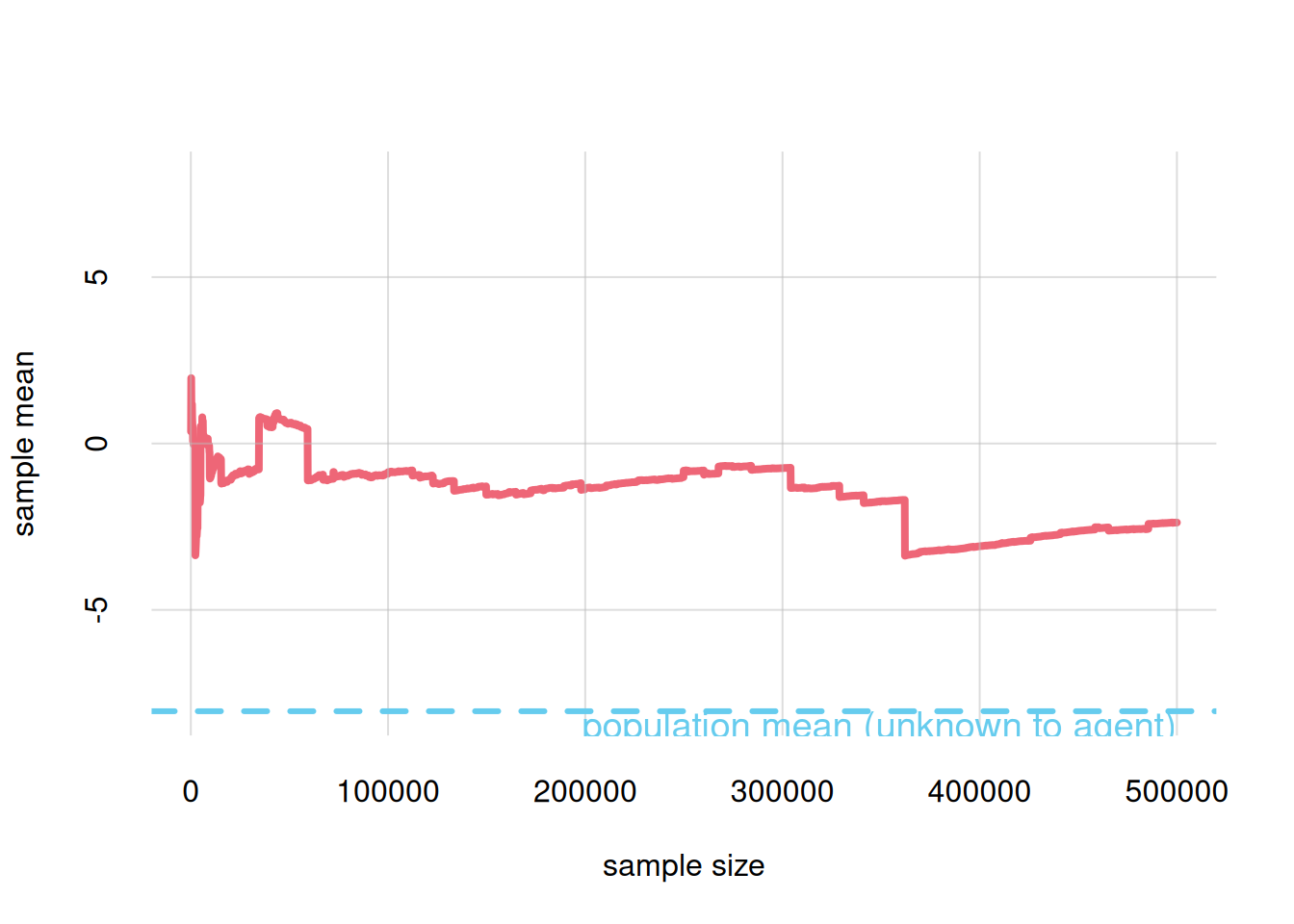
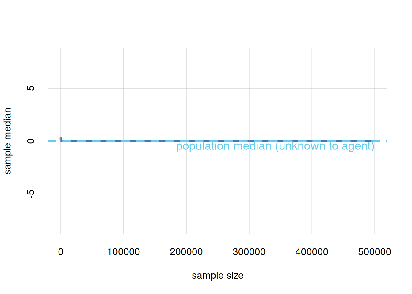
For some populations, the mean and standard deviation calculated in a sample can be wildly different from those of the full population – even when the sample comprises half of the full population! This does not happen with the median and quartiles. Here is a demonstration in R. Try it out in your favourite programming language.

Guided exercise

We imagine to have a population of 1 000 000 units. These units have continuous interval variates \(X\) and \(Y\), each with an approximately standard Gaussian frequency distribution. These variates are not actual part of the population definition, however. Rather, an agent only has access to, or maybe it’s only interested in, the ratio of these two variates \(T \coloneqq X/Y\).

The agent is in particular interested in the mean of the variate \(T\) in the full population, but has only access to the values of \(T\) in a sample. How does the mean calculated from a sample of increasing size compare with the actual mean of the full population? For comparison, we also study the median of the full population and of the samples.

First let’s create the values of the variates \(X\) and \(Y\), and construct \(T\) from them:

## Load custom plot functions
source('code/tplotfunctions.R')
set.seed(1000) # to reproduce results

N <- 1000000 # population size

X <- rnorm(N) # variate invisible to agent
Y <- rnorm(N) # variate invisible to agent

T <- X/Y # variate considered by agent

## mean and median of T in the full population
popmean <- mean(T)
cat('\nThe full-population mean is', popmean, '(unknown to the agent)\n')

The full-population mean is -8.04481 (unknown to the agent)
popmedian <- median(T)
cat('\nThe full-population median is', popmedian, '(unknown to the agent)\n')

The full-population median is 0.00188701 (unknown to the agent)

Now we imagine that the agent accumulates samples from the population, starting from 100, increasing by 100 units, until half of the population has been sampled. At each sample increase the agent calculates the sample mean. We plot how the sample mean changes with the sample size. We also plot indicate the full-population mean, which the agent doesn’t know and is trying to guess:

## sizes of successive samples
samplesizes <- seq(100, N/2, by=100)

## empty vectors to contain the means and medians of the increasing samples
samplemeans <- numeric(length(samplesizes))
samplemedians <- numeric(length(samplesizes))

## loop through the increasing samples, calculate mean for each
for(sample in 1:length(samplesizes)){
    samplemeans[sample] <- mean(T[1:samplesizes[sample]])
    samplemedians[sample] <- median(T[1:samplesizes[sample]])

}

## plot how sample means change with sample size, and the actual population mean
commonmax <- 1.01*max(abs(c(popmean,popmedian,samplemeans,samplemedians)))
tplot(x=samplesizes, y=samplemeans,
      xlab='sample size', ylab='sample mean',
      col=2, lwd=4,
      ylim=c(-commonmax,commonmax))
abline(h=popmean, lty=2, lwd=3, col=7)
text(y=popmean, x=max(samplesizes), labels='population mean (unknown to agent)', adj=c(1,1), col=7, cex=1.2)

## plot how sample medians change with sample size, and the actual population median
tplot(x=samplesizes, y=samplemedians,
      xlab='sample size', ylab='sample median',
      col=3, lwd=4,
      ylim=c(-commonmax,commonmax))
abline(h=popmedian, lty=2, lwd=3, col=7)
text(y=popmedian, x=max(samplesizes), labels='population median (unknown to agent)', adj=c(1,1), col=7, cex=1.2)

Test this again with several pseudorandom seeds.


  • Now try a similar exercise but for the standard deviation of \(T\)