28 Example of belief over frequencies: the Dirichlet-mixture distribution

Published

2025-10-27

28.1 A belief distribution for frequencies over nominal variates

There are infinite possible ways to choose a belief distribution \(\mathrm{P}(F\mathclose{}\mathord{\nonscript\mkern 0mu\textrm{\small=}\nonscript\mkern 0mu}\mathopen{}\boldsymbol{f}\nonscript\:\vert\nonscript\:\mathopen{}\mathsfit{I})\) over frequencies. In this chapter we discuss one, called the Dirichlet-mixture belief distribution, in some detail. The state of knowledge underlying this distribution will be denoted \(\mathsfit{I}_{\textrm{d}}\).

The Dirichlet-mixture distribution is appropriate for statistical populations with nominal, discrete variates, or joint variates with all nominal components. It is not appropriate to discrete ordinal variates, because it implicitly assumes that there is no natural order to the variate values.

For the extra curious

Some of the theoretical basis for the choice of this belief distribution can be found in chapters 4–5 of The Estimation of Probabilities.

Suppose we have a simple or joint nominal variate \({\color[RGB]{68,119,170}Z}\) which can take on \(M\) different possible values; these can be joint values, as in the examples of § 24.2. As usual \(\boldsymbol{f}\) denotes a specific frequency distribution for the variate values. For a given value \({\color[RGB]{68,119,170}z}\), we denote by \(f({\color[RGB]{68,119,170}z})\) the relative frequency with which that value occurs in the full population.

The Dirichlet-mixture distribution assigns to \(\boldsymbol{f}\) a probability density given by the following formula:

\[\mathrm{p}(F\mathclose{}\mathord{\nonscript\mkern 0mu\textrm{\small=}\nonscript\mkern 0mu}\mathopen{}\boldsymbol{f}\nonscript\:\vert\nonscript\:\mathopen{} \mathsfit{I}_{\textrm{d}}) = \frac{1}{k_{\text{ma}}-k_{\text{mi}}+1} \sum_{k=k_{\text{mi}}}^{k_{\text{ma}}} \Biggl[\prod_{{\color[RGB]{68,119,170}z}} f({\color[RGB]{68,119,170}z})^{\frac{2^k}{M} -1} \Biggr] \cdot \frac{ \bigl(2^{k} -1 \bigr)! }{ {\bigl(\frac{2^{k}}{M} - 1\bigr)!}^M } \tag{28.1}\]

Besides some multiplicative constants, the probability of a particular frequency distribution is simply proportional to the product of all its individual frequencies, raised to some powers. The product “\(\prod_{{\color[RGB]{68,119,170}z}}\)” is over all \(M\) possible values of \({\color[RGB]{68,119,170}Z}\). The sum “\(\sum_{k}\)” is over an integer (positive or negative) index \(k\) that runs between the minimum value \(k_{\text{mi}}\) and the maximum value \(k_{\text{ma}}\). In the applications of the next chapters these minimum and maximum are chosen as follows:

\[ k_{\text{mi}}=0 \qquad k_{\text{ma}}=20 \]

so the sum “\(\sum_k\)” runs over 21 terms. In most applications it does not matter if we take a lower \(k_{\text{mi}}\) or a higher \(k_{\text{ma}}\).

Meaning of the \(k_{\text{mi}}, k_{\text{ma}}\) parameters

The parameters \(k_{\text{mi}}, k_{\text{ma}}\) encode, approximately speaking, the agent’s built-in belief about how many data are needed to change its initial beliefs. More precisely, \(2^{k_{\text{mi}}}\) and \(2^{k_{\text{ma}}}\) represent a lower and an upper bound on the amount of data necessary to overcome initial beliefs. Values \(k_{\text{mi}}=0\), \(k_{\text{ma}}=20\) represent the belief that such amount could be anywhere between 1 unit and approximately 1 million units. The belief is spread out uniformly across the orders of magnitude in between.

If \(2^{k_{\text{mi}}}\) is larger than the amount of training data, the agent will consider these data insufficient, and tend to give uniform probabilities to its inferences, for example a 50%/50% probability to a binary variate.

If the amount of data that should be considered “enough” is known, for example from previous studies on similar populations, the parameters \(k_{\text{mi}},k_{\text{ma}}\) can be set to that order of magnitude, in base 2, minus or plus some magnitude range.

Note that if such an order of magnitude is not known, then it does not make sense to “estimate” it from training data with other methods, because an agent with a Dirichlet-mixture belief will already do that internally and in an optimal way, provided an ample range is given with \(k_{\text{mi}}, k_{\text{ma}}\).

Exercise 28.1

In the calculations and exercises that follow, try also other \(k_{\text{mi}}\) and \(k_{\text{ma}}\) values, and see what happens.

Let’s see how this formula looks like in a concrete, simple example: the Mars-prospecting scenario, which has many analogies with coin tosses.

The variate \(R\) can take on two values \(\set{{\color[RGB]{102,204,238}{\small\verb;Y;}},{\color[RGB]{204,187,68}{\small\verb;N;}}}\), so \(M=2\) in this case. The frequency distribution consists in two frequencies:

\[f({\color[RGB]{102,204,238}{\small\verb;Y;}}) \qquad f({\color[RGB]{204,187,68}{\small\verb;N;}})\]

of which only one can be chosen independently, since they must sum up to 1. For instance we could consider \(f({\color[RGB]{102,204,238}{\small\verb;Y;}})=0.5, f({\color[RGB]{204,187,68}{\small\verb;N;}})=0.5\), or \(f({\color[RGB]{102,204,238}{\small\verb;Y;}})=0.84, f({\color[RGB]{204,187,68}{\small\verb;N;}})=0.16\), and so on.

In the present example we choose

\[k_{\text{mi}}=0 \qquad k_{\text{ma}}=2\]

so that the sum “\(\sum_k\)” runs over 3 terms.

Let’s use these specific values of \(M\), \(k_{\text{mi}}\), \(k_{\text{ma}}\) in the agent’s belief distribution for the frequencies, and simplify its expression a little:

\[ \begin{aligned} \mathrm{p}(F\mathclose{}\mathord{\nonscript\mkern 0mu\textrm{\small=}\nonscript\mkern 0mu}\mathopen{}\boldsymbol{f}\nonscript\:\vert\nonscript\:\mathopen{} \mathsfit{I}_{\textrm{d}}) &= \frac{1}{2-0+1} \sum_{k=0}^{2} \Biggl[\prod_{{\color[RGB]{68,119,170}z}={\color[RGB]{102,204,238}{\small\verb;Y;}}}^{{\color[RGB]{204,187,68}{\small\verb;N;}}} f({\color[RGB]{68,119,170}z})^{\frac{2^k}{2} -1} \Biggr] \cdot \frac{ \bigl(2^{k} -1 \bigr)! }{ {\bigl(\frac{2^{k}}{2} - 1\bigr)!}^2 } \\[2ex] &= \frac{1}{3} \Biggl[ f({\color[RGB]{102,204,238}{\small\verb;Y;}})^{\frac{2^{0}}{2}-1}\cdot f({\color[RGB]{204,187,68}{\small\verb;N;}})^{\frac{2^{0}}{2}-1} \cdot \frac{ \bigl(2^{0} -1 \bigr)! }{ {\bigl(\frac{2^{0}}{2} - 1\bigr)!}^2 } +{} \\[1ex]&\qquad f({\color[RGB]{102,204,238}{\small\verb;Y;}})^{\frac{2^{1}}{2}-1}\cdot f({\color[RGB]{204,187,68}{\small\verb;N;}})^{\frac{2^{1}}{2}-1} \cdot \frac{ \bigl(2^{1} -1 \bigr)! }{ {\bigl(\frac{2^{1}}{2} - 1\bigr)!}^2 } +{} \\[1ex]&\qquad f({\color[RGB]{102,204,238}{\small\verb;Y;}})^{\frac{2^{2}}{2}-1}\cdot f({\color[RGB]{204,187,68}{\small\verb;N;}})^{\frac{2^{2}}{2}-1} \cdot \frac{ \bigl(2^{2} -1 \bigr)! }{ {\bigl(\frac{2^{2}}{2} - 1\bigr)!}^2 } \Biggr] \\[2ex] &= \frac{1}{3} \Biggl[ \frac{1}{\sqrt{f({\color[RGB]{102,204,238}{\small\verb;Y;}})}}\cdot \frac{1}{\sqrt{f({\color[RGB]{204,187,68}{\small\verb;N;}})}} \cdot \frac{1}{\pi} +{} \\[1ex]&\qquad 1 \cdot 1 \cdot \frac{1}{1} +{} \\[1ex]&\qquad f({\color[RGB]{102,204,238}{\small\verb;Y;}})\cdot f({\color[RGB]{204,187,68}{\small\verb;N;}}) \cdot \frac{6}{1} \Biggr] \\[2ex] &= \frac{1}{3\pi} \cdot \frac{1}{\sqrt{f({\color[RGB]{102,204,238}{\small\verb;Y;}})}}\cdot \frac{1}{\sqrt{f({\color[RGB]{204,187,68}{\small\verb;N;}})}} + \frac{1}{3} + 3 \cdot f({\color[RGB]{102,204,238}{\small\verb;Y;}})\cdot f({\color[RGB]{204,187,68}{\small\verb;N;}}) \end{aligned} \]

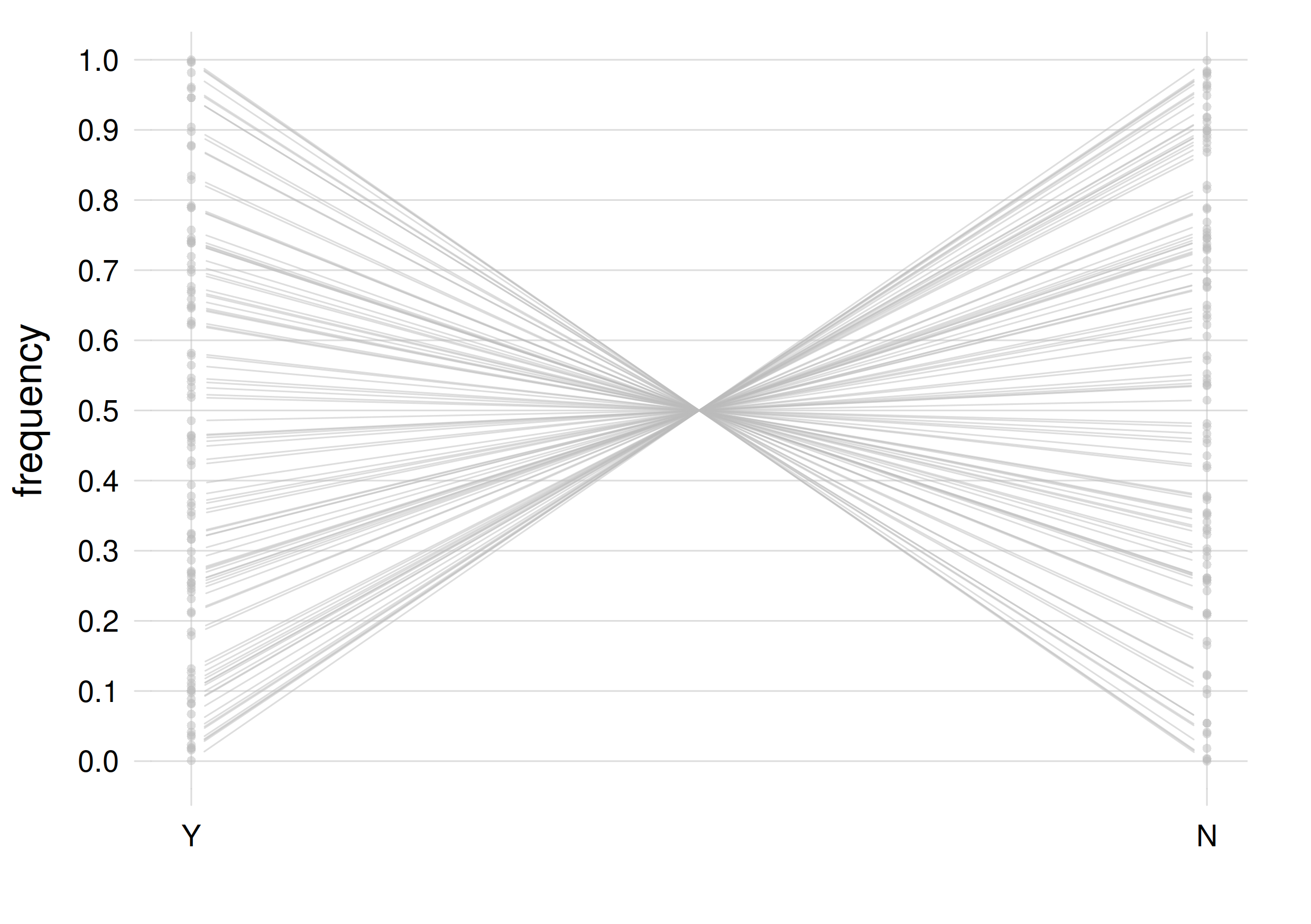
We can visualize this belief distribution (with \(k_{\text{mi}}=0, k_{\text{ma}}=2\)) with a generalized scatter plot (§ 15.7) of 100 frequency distributions; each distribution is represented by a line (recall § 14.2):

Alternatively we can represent the probability density of the frequency \(f({\color[RGB]{102,204,238}{\small\verb;Y;}})\):

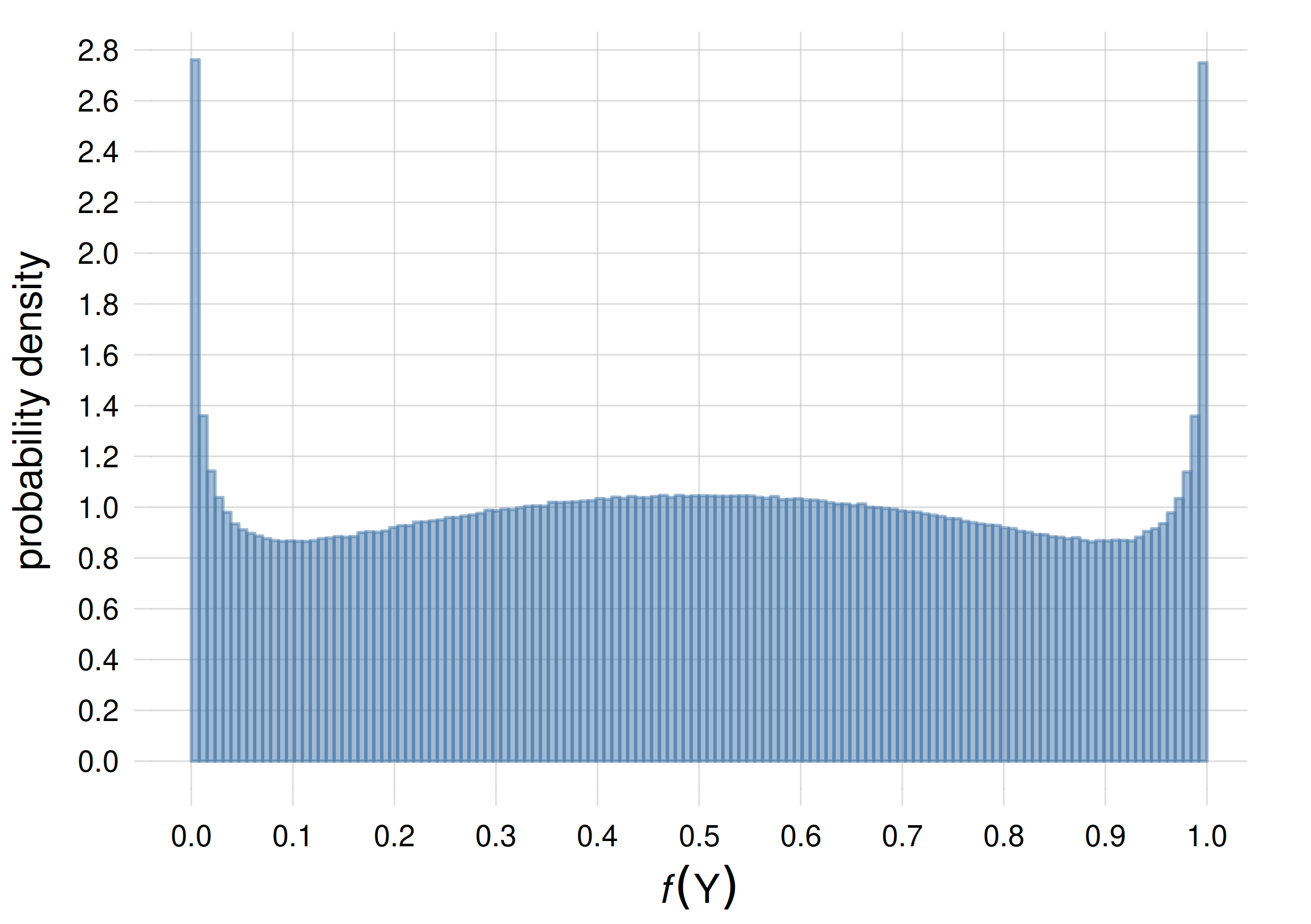
You can see some characteristics of this belief:

all possible frequency distributions are taken into account, that is, no frequency is judged impossible and given zero probability
a higher probability is given to frequency distributions that are almost 50%/50%, or that are almost 0%/100% or 100%/0%

The second characteristic expresses the belief that the agent may more often deal with tasks where frequencies are almost symmetric (think of coin toss), or the opposite: tasks where, once you observe a phenomenon, you’re quite sure you’ll keep observing it. This latter case is typical of some physical phenomena; an example is given by Jaynes:

For example, in a chemical laboratory we find a jar containing an unknown and unlabeled compound. We are at first completely ignorant as to whether a small sample of this compound will dissolve in water or not. But having observed that one small sample does dissolve, we infer immediately that all samples of this compound are water soluble, and although this conclusion does not carry quite the force of deductive proof, we feel strongly that the inference was justified.

For the extra curious

Prior probabilities

Exercise 28.2

Calculate the formula above for these three frequency distributions:

1. \(f({\color[RGB]{102,204,238}{\small\verb;Y;}})=0.5\quad f({\color[RGB]{204,187,68}{\small\verb;N;}})=0.5\)

2. \(f({\color[RGB]{102,204,238}{\small\verb;Y;}})=0.75\quad f({\color[RGB]{204,187,68}{\small\verb;N;}})=0.25\)

3. \(f({\color[RGB]{102,204,238}{\small\verb;Y;}})=0.99\quad f({\color[RGB]{204,187,68}{\small\verb;N;}})=0.01\)

28.2 Examples of inference by a Dirichlet-mixture agent

Degree of belief about a data sequence

Recall that an agent, in order to learn, needs to be initially provided with the full joint belief distribution

\[ \mathrm{P}( \color[RGB]{68,119,170} Z_{L}\mathclose{}\mathord{\nonscript\mkern 0mu\textrm{\small=}\nonscript\mkern 0mu}\mathopen{}z_{L} \mathbin{\mkern-0.5mu,\mkern-0.5mu} \dotsb \mathbin{\mkern-0.5mu,\mkern-0.5mu} Z_{1}\mathclose{}\mathord{\nonscript\mkern 0mu\textrm{\small=}\nonscript\mkern 0mu}\mathopen{}z_1 \color[RGB]{0,0,0} \nonscript\:\vert\nonscript\:\mathopen{} \mathsfit{I} ) \]

where \(L\) is the total number of data that will be used to learn, as well as those that will be subsequently analysed.

A mathematical advantage of the Dirichlet-mixture belief distribution is that it allows us to compute this belief distribution, and several others, in an exact way. Start from de Finetti’s representation theorem (§ 27.1) and use the Dirichlet-mixture (28.1) for \(\mathrm{P}(F\mathclose{}\mathord{\nonscript\mkern 0mu\textrm{\small=}\nonscript\mkern 0mu}\mathopen{}\boldsymbol{f}\nonscript\:\vert\nonscript\:\mathopen{} \mathsfit{I})\). The integral “\(\int\,\mathrm{d}\boldsymbol{f}\)” can be solved explicitly and we find the following result:

\[ \begin{aligned} \mathrm{P}( \color[RGB]{68,119,170} Z_{L}\mathclose{}\mathord{\nonscript\mkern 0mu\textrm{\small=}\nonscript\mkern 0mu}\mathopen{}z_{L} \mathbin{\mkern-0.5mu,\mkern-0.5mu} \dotsb \mathbin{\mkern-0.5mu,\mkern-0.5mu} Z_{1}\mathclose{}\mathord{\nonscript\mkern 0mu\textrm{\small=}\nonscript\mkern 0mu}\mathopen{}z_1 \color[RGB]{0,0,0} \nonscript\:\vert\nonscript\:\mathopen{} \mathsfit{I}_{\textrm{d}} ) &= \int f(\color[RGB]{68,119,170}Z_{L}\mathclose{}\mathord{\nonscript\mkern 0mu\textrm{\small=}\nonscript\mkern 0mu}\mathopen{}z_{L} \color[RGB]{0,0,0}) \cdot \,\dotsb\, \cdot f(\color[RGB]{68,119,170}Z_{1}\mathclose{}\mathord{\nonscript\mkern 0mu\textrm{\small=}\nonscript\mkern 0mu}\mathopen{}z_1 \color[RGB]{0,0,0}) \cdot \mathrm{p}(F\mathclose{}\mathord{\nonscript\mkern 0mu\textrm{\small=}\nonscript\mkern 0mu}\mathopen{}\boldsymbol{f}\nonscript\:\vert\nonscript\:\mathopen{} \mathsfit{I}_{\textrm{d}}) \,\mathrm{d}\boldsymbol{f} \\[2ex] &= \frac{1}{k_{\text{ma}}-k_{\text{mi}}+1} \sum_{k=k_{\text{mi}}}^{k_{\text{ma}}} \frac{ \prod_{{\color[RGB]{68,119,170}z}} \bigl(\frac{2^{k}}{M} + \#{\color[RGB]{68,119,170}z}- 1\bigr)! }{ \bigl(2^{k} + L -1 \bigr)! } \cdot \frac{ \bigl(2^{k} -1 \bigr)! }{ {\bigl(\frac{2^{k}}{M} - 1\bigr)!}^M } \end{aligned} \tag{28.2}\]

where \(\#{\color[RGB]{68,119,170}z}\) is the multiplicity with which the specific value \({\color[RGB]{68,119,170}z}\) occurs in the sequence \(\color[RGB]{68,119,170}z_1,\dotsc,z_{L}\).

To understand better the formula above, let’s use it in an example from the Mars-prospecting scenario of ch. 25. Take the sequence¹

¹ Remember that the agent has exchangeable beliefs, so the units’ IDs don’t matter (§ 25.3)!

\[ R_1\mathclose{}\mathord{\nonscript\mkern 0mu\textrm{\small=}\nonscript\mkern 0mu}\mathopen{}{\color[RGB]{102,204,238}{\small\verb;Y;}}\mathbin{\mkern-0.5mu,\mkern-0.5mu}R_2\mathclose{}\mathord{\nonscript\mkern 0mu\textrm{\small=}\nonscript\mkern 0mu}\mathopen{}{\color[RGB]{102,204,238}{\small\verb;Y;}}\mathbin{\mkern-0.5mu,\mkern-0.5mu}R_3\mathclose{}\mathord{\nonscript\mkern 0mu\textrm{\small=}\nonscript\mkern 0mu}\mathopen{}{\color[RGB]{204,187,68}{\small\verb;N;}}\mathbin{\mkern-0.5mu,\mkern-0.5mu}R_4\mathclose{}\mathord{\nonscript\mkern 0mu\textrm{\small=}\nonscript\mkern 0mu}\mathopen{}{\color[RGB]{102,204,238}{\small\verb;Y;}} \]

In this sequence of four values, value \({\color[RGB]{102,204,238}{\small\verb;Y;}}\) appears thrice and value \({\color[RGB]{204,187,68}{\small\verb;N;}}\) once. So in this case we have

\[\#{\color[RGB]{102,204,238}{\small\verb;Y;}}= 3\ ,\qquad \#{\color[RGB]{204,187,68}{\small\verb;N;}}= 1 \ ,\qquad L = 4\ .\]

We also have \(M=2\) (two possible distinct values), and we still take \(k_{\text{mi}}=0, k_{\text{ma}}=2\). The formula above then gives

\[ \begin{aligned} &\mathrm{P}( \underbracket[0.1ex]{R_1\mathclose{}\mathord{\nonscript\mkern 0mu\textrm{\small=}\nonscript\mkern 0mu}\mathopen{}{\color[RGB]{102,204,238}{\small\verb;Y;}}\mathbin{\mkern-0.5mu,\mkern-0.5mu}R_2\mathclose{}\mathord{\nonscript\mkern 0mu\textrm{\small=}\nonscript\mkern 0mu}\mathopen{}{\color[RGB]{102,204,238}{\small\verb;Y;}}\mathbin{\mkern-0.5mu,\mkern-0.5mu}R_3\mathclose{}\mathord{\nonscript\mkern 0mu\textrm{\small=}\nonscript\mkern 0mu}\mathopen{}{\color[RGB]{204,187,68}{\small\verb;N;}}\mathbin{\mkern-0.5mu,\mkern-0.5mu}R_4\mathclose{}\mathord{\nonscript\mkern 0mu\textrm{\small=}\nonscript\mkern 0mu}\mathopen{}{\color[RGB]{102,204,238}{\small\verb;Y;}}}_{ \color[RGB]{187,187,187}L=4\quad \#{\small\verb;Y;}=3\quad \#{\small\verb;N;}=1 } \nonscript\:\vert\nonscript\:\mathopen{} \mathsfit{I}_{\textrm{d}} ) \\ &\qquad{}= \frac{1}{k_{\text{ma}}-k_{\text{mi}}+1} \sum_{k=k_{\text{mi}}}^{k_{\text{ma}}} \frac{ \prod_{{\color[RGB]{68,119,170}z}} \bigl(\frac{2^{k}}{M} + \#{\color[RGB]{68,119,170}z}- 1\bigr)! }{ \bigl(2^{k} + L -1 \bigr)! } \cdot \frac{ \bigl(2^{k} -1 \bigr)! }{ {\bigl(\frac{2^{k}}{M} - 1\bigr)!}^M } \\[2ex] &\qquad{}= \frac{1}{2-0+1} \sum_{k=0}^{2} \frac{ \bigl(\frac{2^{k}}{2} + \#{\color[RGB]{102,204,238}{\small\verb;Y;}}- 1\bigr)! \cdot \bigl(\frac{2^{k}}{2} + \#{\color[RGB]{204,187,68}{\small\verb;N;}}- 1\bigr)! }{ \bigl(2^{k} + 4 -1 \bigr)! } \cdot \frac{ \bigl(2^{k} -1 \bigr)! }{ {\bigl(\frac{2^{k}}{2} - 1\bigr)!}^2 } \\[2ex] &\qquad{}= \frac{1}{3} \sum_{k=0}^{2} \frac{ \bigl(\frac{2^{k}}{2} + {\color[RGB]{102,204,238}3} - 1\bigr)! \cdot \bigl(\frac{2^{k}}{2} + {\color[RGB]{204,187,68}1} - 1\bigr)! }{ \bigl(2^{k} + 3 \bigr)! } \cdot \frac{ \bigl(2^{k} -1 \bigr)! }{ {\bigl(\frac{2^{k}}{2} - 1\bigr)!}^2 } \\[1ex] &\qquad{}= \boldsymbol{0.048 735 1} \end{aligned} \]

Exercise 28.3

Implement the calculation above in your favourite programming language.
Using the formula above, calculate:
- \(\mathrm{P}(R_1\mathclose{}\mathord{\nonscript\mkern 0mu\textrm{\small=}\nonscript\mkern 0mu}\mathopen{}{\color[RGB]{102,204,238}{\small\verb;Y;}}\nonscript\:\vert\nonscript\:\mathopen{} \mathsfit{I}_{\textrm{d}})\) . Does the result make sense?
- \(\mathrm{P}(R_{32}\mathclose{}\mathord{\nonscript\mkern 0mu\textrm{\small=}\nonscript\mkern 0mu}\mathopen{}{\color[RGB]{204,187,68}{\small\verb;N;}}\mathbin{\mkern-0.5mu,\mkern-0.5mu}R_{102}\mathclose{}\mathord{\nonscript\mkern 0mu\textrm{\small=}\nonscript\mkern 0mu}\mathopen{}{\color[RGB]{204,187,68}{\small\verb;N;}}\mathbin{\mkern-0.5mu,\mkern-0.5mu}R_{8}\mathclose{}\mathord{\nonscript\mkern 0mu\textrm{\small=}\nonscript\mkern 0mu}\mathopen{}{\color[RGB]{204,187,68}{\small\verb;N;}}\nonscript\:\vert\nonscript\:\mathopen{} \mathsfit{I}_{\textrm{d}})\)

Try doing the calculation above on a computer with \(k_{\text{mi}}=0, k_{\text{ma}}=20\). What happens?

Using formula (28.2) we can solve all the kinds of task discussed in § 24.2. Let’s see a couple of simple examples.

Example 1: Forecast about one variate, given previous observations

In the following example we consider only one predictand variate \(R\): the presence of haematite. There are no predictors. The Dirichlet-mixture agent observes the value of this variate in several rocks, and tries to forecast its value in a new rock. The variate of the population of interest has two possible values, in formula (28.2) we have \(M=2\). We still take \(k_{\text{mi}}=0\), \(k_{\text{ma}}=2\).

The agent has collected three rocks. Upon examination, two of them contain haematite, one doesn’t. The agent’s data are therefore

\[\text{\small data:}\quad R_1\mathclose{}\mathord{\nonscript\mkern 0mu\textrm{\small=}\nonscript\mkern 0mu}\mathopen{}{\color[RGB]{102,204,238}{\small\verb;Y;}}\mathbin{\mkern-0.5mu,\mkern-0.5mu}R_2\mathclose{}\mathord{\nonscript\mkern 0mu\textrm{\small=}\nonscript\mkern 0mu}\mathopen{}{\color[RGB]{102,204,238}{\small\verb;Y;}}\mathbin{\mkern-0.5mu,\mkern-0.5mu}R_3\mathclose{}\mathord{\nonscript\mkern 0mu\textrm{\small=}\nonscript\mkern 0mu}\mathopen{}{\color[RGB]{204,187,68}{\small\verb;N;}}\]

What belief should the agent have about finding haematite in a newly collected rock? That is, what value should it assign to the probability

\[\mathrm{P}(R_4\mathclose{}\mathord{\nonscript\mkern 0mu\textrm{\small=}\nonscript\mkern 0mu}\mathopen{}{\color[RGB]{102,204,238}{\small\verb;Y;}}\nonscript\:\vert\nonscript\:\mathopen{} R_1\mathclose{}\mathord{\nonscript\mkern 0mu\textrm{\small=}\nonscript\mkern 0mu}\mathopen{}{\color[RGB]{102,204,238}{\small\verb;Y;}}\mathbin{\mkern-0.5mu,\mkern-0.5mu}R_2\mathclose{}\mathord{\nonscript\mkern 0mu\textrm{\small=}\nonscript\mkern 0mu}\mathopen{}{\color[RGB]{102,204,238}{\small\verb;Y;}}\mathbin{\mkern-0.5mu,\mkern-0.5mu}R_3\mathclose{}\mathord{\nonscript\mkern 0mu\textrm{\small=}\nonscript\mkern 0mu}\mathopen{}{\color[RGB]{204,187,68}{\small\verb;N;}}\mathbin{\mkern-0.5mu,\mkern-0.5mu}\mathsfit{I}_{\textrm{d}})\ ?\]

This conditional probability is given by

\[ \begin{aligned} &\mathrm{P}(R_4\mathclose{}\mathord{\nonscript\mkern 0mu\textrm{\small=}\nonscript\mkern 0mu}\mathopen{}{\color[RGB]{102,204,238}{\small\verb;Y;}}\nonscript\:\vert\nonscript\:\mathopen{} R_1\mathclose{}\mathord{\nonscript\mkern 0mu\textrm{\small=}\nonscript\mkern 0mu}\mathopen{}{\color[RGB]{102,204,238}{\small\verb;Y;}}\mathbin{\mkern-0.5mu,\mkern-0.5mu}R_2\mathclose{}\mathord{\nonscript\mkern 0mu\textrm{\small=}\nonscript\mkern 0mu}\mathopen{}{\color[RGB]{102,204,238}{\small\verb;Y;}}\mathbin{\mkern-0.5mu,\mkern-0.5mu}R_3\mathclose{}\mathord{\nonscript\mkern 0mu\textrm{\small=}\nonscript\mkern 0mu}\mathopen{}{\color[RGB]{204,187,68}{\small\verb;N;}}\mathbin{\mkern-0.5mu,\mkern-0.5mu}\mathsfit{I}_{\textrm{d}}) \\[1ex] &\qquad{}= \frac{ \mathrm{P}(R_4\mathclose{}\mathord{\nonscript\mkern 0mu\textrm{\small=}\nonscript\mkern 0mu}\mathopen{}{\color[RGB]{102,204,238}{\small\verb;Y;}}\mathbin{\mkern-0.5mu,\mkern-0.5mu}R_1\mathclose{}\mathord{\nonscript\mkern 0mu\textrm{\small=}\nonscript\mkern 0mu}\mathopen{}{\color[RGB]{102,204,238}{\small\verb;Y;}}\mathbin{\mkern-0.5mu,\mkern-0.5mu}R_2\mathclose{}\mathord{\nonscript\mkern 0mu\textrm{\small=}\nonscript\mkern 0mu}\mathopen{}{\color[RGB]{102,204,238}{\small\verb;Y;}}\mathbin{\mkern-0.5mu,\mkern-0.5mu}R_3\mathclose{}\mathord{\nonscript\mkern 0mu\textrm{\small=}\nonscript\mkern 0mu}\mathopen{}{\color[RGB]{204,187,68}{\small\verb;N;}}\nonscript\:\vert\nonscript\:\mathopen{} \mathsfit{I}_{\textrm{d}}) }{ \sum_{{\color[RGB]{170,51,119}r}={\color[RGB]{102,204,238}{\small\verb;Y;}}}^{{\color[RGB]{204,187,68}{\small\verb;N;}}} \mathrm{P}(R_4\mathclose{}\mathord{\nonscript\mkern 0mu\textrm{\small=}\nonscript\mkern 0mu}\mathopen{}{\color[RGB]{170,51,119}r} \mathbin{\mkern-0.5mu,\mkern-0.5mu}R_1\mathclose{}\mathord{\nonscript\mkern 0mu\textrm{\small=}\nonscript\mkern 0mu}\mathopen{}{\color[RGB]{102,204,238}{\small\verb;Y;}}\mathbin{\mkern-0.5mu,\mkern-0.5mu}R_2\mathclose{}\mathord{\nonscript\mkern 0mu\textrm{\small=}\nonscript\mkern 0mu}\mathopen{}{\color[RGB]{102,204,238}{\small\verb;Y;}}\mathbin{\mkern-0.5mu,\mkern-0.5mu}R_3\mathclose{}\mathord{\nonscript\mkern 0mu\textrm{\small=}\nonscript\mkern 0mu}\mathopen{}{\color[RGB]{204,187,68}{\small\verb;N;}}\nonscript\:\vert\nonscript\:\mathopen{} \mathsfit{I}_{\textrm{d}}) } \\[1ex] &\qquad{}\equiv \frac{ \mathrm{P}(R_4\mathclose{}\mathord{\nonscript\mkern 0mu\textrm{\small=}\nonscript\mkern 0mu}\mathopen{}{\color[RGB]{102,204,238}{\small\verb;Y;}}\, \mathbin{\mkern-0.5mu,\mkern-0.5mu}\, R_1\mathclose{}\mathord{\nonscript\mkern 0mu\textrm{\small=}\nonscript\mkern 0mu}\mathopen{}{\color[RGB]{102,204,238}{\small\verb;Y;}}\mathbin{\mkern-0.5mu,\mkern-0.5mu}R_2\mathclose{}\mathord{\nonscript\mkern 0mu\textrm{\small=}\nonscript\mkern 0mu}\mathopen{}{\color[RGB]{102,204,238}{\small\verb;Y;}}\mathbin{\mkern-0.5mu,\mkern-0.5mu}R_3\mathclose{}\mathord{\nonscript\mkern 0mu\textrm{\small=}\nonscript\mkern 0mu}\mathopen{}{\color[RGB]{204,187,68}{\small\verb;N;}}\nonscript\:\vert\nonscript\:\mathopen{} \mathsfit{I}_{\textrm{d}}) }{ \mathrm{P}(R_4\mathclose{}\mathord{\nonscript\mkern 0mu\textrm{\small=}\nonscript\mkern 0mu}\mathopen{}{\color[RGB]{102,204,238}{\small\verb;Y;}}\, \mathbin{\mkern-0.5mu,\mkern-0.5mu}\, R_1\mathclose{}\mathord{\nonscript\mkern 0mu\textrm{\small=}\nonscript\mkern 0mu}\mathopen{}{\color[RGB]{102,204,238}{\small\verb;Y;}}\mathbin{\mkern-0.5mu,\mkern-0.5mu}R_2\mathclose{}\mathord{\nonscript\mkern 0mu\textrm{\small=}\nonscript\mkern 0mu}\mathopen{}{\color[RGB]{102,204,238}{\small\verb;Y;}}\mathbin{\mkern-0.5mu,\mkern-0.5mu}R_3\mathclose{}\mathord{\nonscript\mkern 0mu\textrm{\small=}\nonscript\mkern 0mu}\mathopen{}{\color[RGB]{204,187,68}{\small\verb;N;}}\nonscript\:\vert\nonscript\:\mathopen{} \mathsfit{I}_{\textrm{d}}) + \mathrm{P}(R_4\mathclose{}\mathord{\nonscript\mkern 0mu\textrm{\small=}\nonscript\mkern 0mu}\mathopen{}{\color[RGB]{204,187,68}{\small\verb;N;}}\, \mathbin{\mkern-0.5mu,\mkern-0.5mu}\, R_1\mathclose{}\mathord{\nonscript\mkern 0mu\textrm{\small=}\nonscript\mkern 0mu}\mathopen{}{\color[RGB]{102,204,238}{\small\verb;Y;}}\mathbin{\mkern-0.5mu,\mkern-0.5mu}R_2\mathclose{}\mathord{\nonscript\mkern 0mu\textrm{\small=}\nonscript\mkern 0mu}\mathopen{}{\color[RGB]{102,204,238}{\small\verb;Y;}}\mathbin{\mkern-0.5mu,\mkern-0.5mu}R_3\mathclose{}\mathord{\nonscript\mkern 0mu\textrm{\small=}\nonscript\mkern 0mu}\mathopen{}{\color[RGB]{204,187,68}{\small\verb;N;}}\nonscript\:\vert\nonscript\:\mathopen{} \mathsfit{I}_{\textrm{d}}) } \end{aligned} \]

and we can calculate the probabilities at the numerator and denominators using formula (28.2):

– The fraction above requires the computation of two joint probabilities:

\[ \begin{aligned} \mathrm{P}(R_4\mathclose{}\mathord{\nonscript\mkern 0mu\textrm{\small=}\nonscript\mkern 0mu}\mathopen{}{\color[RGB]{102,204,238}{\small\verb;Y;}}\, \mathbin{\mkern-0.5mu,\mkern-0.5mu}\, R_1\mathclose{}\mathord{\nonscript\mkern 0mu\textrm{\small=}\nonscript\mkern 0mu}\mathopen{}{\color[RGB]{102,204,238}{\small\verb;Y;}}\mathbin{\mkern-0.5mu,\mkern-0.5mu}R_2\mathclose{}\mathord{\nonscript\mkern 0mu\textrm{\small=}\nonscript\mkern 0mu}\mathopen{}{\color[RGB]{102,204,238}{\small\verb;Y;}}\mathbin{\mkern-0.5mu,\mkern-0.5mu}R_3\mathclose{}\mathord{\nonscript\mkern 0mu\textrm{\small=}\nonscript\mkern 0mu}\mathopen{}{\color[RGB]{204,187,68}{\small\verb;N;}}\nonscript\:\vert\nonscript\:\mathopen{} \mathsfit{I}_{\textrm{d}}) \\[1ex] \mathrm{P}(R_4\mathclose{}\mathord{\nonscript\mkern 0mu\textrm{\small=}\nonscript\mkern 0mu}\mathopen{}{\color[RGB]{204,187,68}{\small\verb;N;}}\, \mathbin{\mkern-0.5mu,\mkern-0.5mu}\, R_1\mathclose{}\mathord{\nonscript\mkern 0mu\textrm{\small=}\nonscript\mkern 0mu}\mathopen{}{\color[RGB]{102,204,238}{\small\verb;Y;}}\mathbin{\mkern-0.5mu,\mkern-0.5mu}R_2\mathclose{}\mathord{\nonscript\mkern 0mu\textrm{\small=}\nonscript\mkern 0mu}\mathopen{}{\color[RGB]{102,204,238}{\small\verb;Y;}}\mathbin{\mkern-0.5mu,\mkern-0.5mu}R_3\mathclose{}\mathord{\nonscript\mkern 0mu\textrm{\small=}\nonscript\mkern 0mu}\mathopen{}{\color[RGB]{204,187,68}{\small\verb;N;}}\nonscript\:\vert\nonscript\:\mathopen{} \mathsfit{I}_{\textrm{d}}) \end{aligned} \]

Note how they are associated with the two possible hypotheses about the new rock:

\[R_4\mathclose{}\mathord{\nonscript\mkern 0mu\textrm{\small=}\nonscript\mkern 0mu}\mathopen{}{\color[RGB]{102,204,238}{\small\verb;Y;}}\,? \qquad R_4\mathclose{}\mathord{\nonscript\mkern 0mu\textrm{\small=}\nonscript\mkern 0mu}\mathopen{}{\color[RGB]{204,187,68}{\small\verb;N;}}\,?\]

of which the first one interests us.

– In the first joint probability, \({\color[RGB]{102,204,238}{\small\verb;Y;}}\) appears thrice and \({\color[RGB]{204,187,68}{\small\verb;N;}}\) appears once, so

\[\#{\color[RGB]{102,204,238}{\small\verb;Y;}}= 3\ ,\qquad \#{\color[RGB]{204,187,68}{\small\verb;N;}}= 1\ ,\qquad {\color[RGB]{119,119,119}L} = {\color[RGB]{119,119,119}4}\ .\]

Formula (28.2) gives

– In the second joint probability, \({\color[RGB]{102,204,238}{\small\verb;Y;}}\) appears twice and \({\color[RGB]{204,187,68}{\small\verb;N;}}\) appears twice, so

\[\#{\color[RGB]{102,204,238}{\small\verb;Y;}}= 2\ ,\qquad \#{\color[RGB]{204,187,68}{\small\verb;N;}}= 2\ ,\qquad {\color[RGB]{119,119,119}L} = {\color[RGB]{119,119,119}4}\ .\]

We find

– We can finally substitute the values we just found into the initial fraction. The probability for the hypothesis of interest is

Exercise 28.4

The inference problem above has some analogy with coin tossing: there’s just one, binary, variate. This agent could have been used to make forecasts about coin tosses.

Consider the result above from the point of view of this analogy. Let’s say that \({\color[RGB]{102,204,238}{\small\verb;Y;}}\) would be “heads”, and \({\color[RGB]{204,187,68}{\small\verb;N;}}\) “tails”. Having observed four coin tosses, with three heads and one tail, the agent is giving a 58% probability for heads at the next toss.
- Do you consider this probability reasonable? Why?
- In which different coin-tossing circumstances would you consider this probability reasonable (given the same previous observation data)?
Try doing the calculation above on a computer, using the values \(k_{\text{mi}}=0, k_{\text{ma}}=20\).

If you use the formulae above as they’re given, you’ll probably get just NaNs. The formulae above must be rewritten in a different way in order not to generate overflow. The result would be \(\boldsymbol{51.42\%}\).

Example 2: Forecast given predictor but no previous observations

Let’s go back to the hospital scenario of § 17.5. The units are patients coming into a hospital. The population is characterized by two nominal variates:

\(T\): the patient’s means of transportation at arrival, with domain \(\set{{\small\verb;ambulance;}, {\small\verb;helicopter;}, {\small\verb;other;}}\)
\(U\): the patient’s need of urgent care, with domain \(\set{{\small\verb;urgent;}, {\small\verb;non-urgent;}}\)

The combined variate \((U \mathbin{\mkern-0.5mu,\mkern-0.5mu}T)\) has \(M = 2\cdot 3 = 6\) possible values. We still use parameters \(k_{\text{mi}}=0\) and \(k_{\text{ma}}=2\) in formula (28.2).

The agent’s task is to forecast whether the next incoming patient will require urgent care, given information about the patient’s transportation. Therefore variate \(U\) is the predictand, and \(T\) the predictor.

Two patients previously arrived to the hospital, but for the moment we assume that no information about them was given to the agent. Thus we have a Dirichlet-mixture agent that hasn’t learned anything yet.

A third patient is incoming by ambulance:

\(T_3\mathclose{}\mathord{\nonscript\mkern 0mu\textrm{\small=}\nonscript\mkern 0mu}\mathopen{}{\small\verb;ambulance;}\)

What is the agent’s belief that this patient requires urgent care?

Since no information about the previous patients is available to the agent, its belief is expressed by

\[ \begin{aligned} &\mathrm{P}(U_3\mathclose{}\mathord{\nonscript\mkern 0mu\textrm{\small=}\nonscript\mkern 0mu}\mathopen{}{\small\verb;urgent;}\nonscript\:\vert\nonscript\:\mathopen{} T_3\mathclose{}\mathord{\nonscript\mkern 0mu\textrm{\small=}\nonscript\mkern 0mu}\mathopen{}{\small\verb;ambulance;}\mathbin{\mkern-0.5mu,\mkern-0.5mu}\mathsfit{I}_{\textrm{d}}) \\[1ex] &\qquad {}= \frac{ \mathrm{P}(U_3\mathclose{}\mathord{\nonscript\mkern 0mu\textrm{\small=}\nonscript\mkern 0mu}\mathopen{}{\small\verb;urgent;}\mathbin{\mkern-0.5mu,\mkern-0.5mu}T_3\mathclose{}\mathord{\nonscript\mkern 0mu\textrm{\small=}\nonscript\mkern 0mu}\mathopen{}{\small\verb;ambulance;}\nonscript\:\vert\nonscript\:\mathopen{} \mathsfit{I}_{\textrm{d}}) }{ \sum_{u = {\small\verb;urgent;}}^{{\small\verb;non-urgent;}} \mathrm{P}(U_3\mathclose{}\mathord{\nonscript\mkern 0mu\textrm{\small=}\nonscript\mkern 0mu}\mathopen{}u \mathbin{\mkern-0.5mu,\mkern-0.5mu}T_3\mathclose{}\mathord{\nonscript\mkern 0mu\textrm{\small=}\nonscript\mkern 0mu}\mathopen{}{\small\verb;ambulance;}\nonscript\:\vert\nonscript\:\mathopen{} \mathsfit{I}_{\textrm{d}}) } \\[1ex] &\qquad {}= \frac{ \mathrm{P}(U_3\mathclose{}\mathord{\nonscript\mkern 0mu\textrm{\small=}\nonscript\mkern 0mu}\mathopen{}{\small\verb;urgent;}\mathbin{\mkern-0.5mu,\mkern-0.5mu}T_3\mathclose{}\mathord{\nonscript\mkern 0mu\textrm{\small=}\nonscript\mkern 0mu}\mathopen{}{\small\verb;ambulance;}\nonscript\:\vert\nonscript\:\mathopen{} \mathsfit{I}_{\textrm{d}}) }{ \mathrm{P}(U_3\mathclose{}\mathord{\nonscript\mkern 0mu\textrm{\small=}\nonscript\mkern 0mu}\mathopen{}{\small\verb;urgent;}\mathbin{\mkern-0.5mu,\mkern-0.5mu}T_3\mathclose{}\mathord{\nonscript\mkern 0mu\textrm{\small=}\nonscript\mkern 0mu}\mathopen{}{\small\verb;ambulance;}\nonscript\:\vert\nonscript\:\mathopen{} \mathsfit{I}_{\textrm{d}}) + \mathrm{P}(U_3\mathclose{}\mathord{\nonscript\mkern 0mu\textrm{\small=}\nonscript\mkern 0mu}\mathopen{}{\small\verb;non-urgent;}\mathbin{\mkern-0.5mu,\mkern-0.5mu}T_3\mathclose{}\mathord{\nonscript\mkern 0mu\textrm{\small=}\nonscript\mkern 0mu}\mathopen{}{\small\verb;ambulance;}\nonscript\:\vert\nonscript\:\mathopen{} \mathsfit{I}_{\textrm{d}}) } \end{aligned} \]

– We need to calculate the two joint probabilities

\[ \mathrm{P}(U_3\mathclose{}\mathord{\nonscript\mkern 0mu\textrm{\small=}\nonscript\mkern 0mu}\mathopen{}{\small\verb;urgent;}\mathbin{\mkern-0.5mu,\mkern-0.5mu}T_3\mathclose{}\mathord{\nonscript\mkern 0mu\textrm{\small=}\nonscript\mkern 0mu}\mathopen{}{\small\verb;ambulance;}\nonscript\:\vert\nonscript\:\mathopen{} \mathsfit{I}_{\textrm{d}}) \qquad \mathrm{P}(U_3\mathclose{}\mathord{\nonscript\mkern 0mu\textrm{\small=}\nonscript\mkern 0mu}\mathopen{}{\small\verb;non-urgent;}\mathbin{\mkern-0.5mu,\mkern-0.5mu}T_3\mathclose{}\mathord{\nonscript\mkern 0mu\textrm{\small=}\nonscript\mkern 0mu}\mathopen{}{\small\verb;ambulance;}\nonscript\:\vert\nonscript\:\mathopen{} \mathsfit{I}_{\textrm{d}}) \]

corresponding to the two hypotheses of interest: \(U_3\mathclose{}\mathord{\nonscript\mkern 0mu\textrm{\small=}\nonscript\mkern 0mu}\mathopen{}{\small\verb;urgent;}\) and \(U_3\mathclose{}\mathord{\nonscript\mkern 0mu\textrm{\small=}\nonscript\mkern 0mu}\mathopen{}{\small\verb;non-urgent;}\).

– In the first joint probability, the joint value \((U\mathclose{}\mathord{\nonscript\mkern 0mu\textrm{\small=}\nonscript\mkern 0mu}\mathopen{}{\small\verb;urgent;}\mathbin{\mkern-0.5mu,\mkern-0.5mu}T\mathclose{}\mathord{\nonscript\mkern 0mu\textrm{\small=}\nonscript\mkern 0mu}\mathopen{}{\small\verb;ambulance;})\) appears once, and the remaining five joint values, like \((U\mathclose{}\mathord{\nonscript\mkern 0mu\textrm{\small=}\nonscript\mkern 0mu}\mathopen{}{\small\verb;non-urgent;}\mathbin{\mkern-0.5mu,\mkern-0.5mu}T\mathclose{}\mathord{\nonscript\mkern 0mu\textrm{\small=}\nonscript\mkern 0mu}\mathopen{}{\small\verb;ambulance;})\), \((U\mathclose{}\mathord{\nonscript\mkern 0mu\textrm{\small=}\nonscript\mkern 0mu}\mathopen{}{\small\verb;urgent;}\mathbin{\mkern-0.5mu,\mkern-0.5mu}T\mathclose{}\mathord{\nonscript\mkern 0mu\textrm{\small=}\nonscript\mkern 0mu}\mathopen{}{\small\verb;other;})\), etc., appear zero times:

\[\#({\small\verb;urgent;}, {\small\verb;ambulance;}) = {\color[RGB]{102,204,238}1}\ ,\qquad\text{\small five others }\#(\dotsc,\dotsc) = {\color[RGB]{204,187,68}0}\ ,\qquad {\color[RGB]{119,119,119}L} = {\color[RGB]{119,119,119}1}\ .\]

Formula (28.2) gives

– In the second joint probability, the joint value \((U\mathclose{}\mathord{\nonscript\mkern 0mu\textrm{\small=}\nonscript\mkern 0mu}\mathopen{}{\small\verb;non-urgent;}\mathbin{\mkern-0.5mu,\mkern-0.5mu}T\mathclose{}\mathord{\nonscript\mkern 0mu\textrm{\small=}\nonscript\mkern 0mu}\mathopen{}{\small\verb;ambulance;})\) appears once, and the remaining five joint values appear zero times:

\[\#({\small\verb;non-urgent;}, {\small\verb;ambulance;}) = {\color[RGB]{102,204,238}1}\ ,\qquad\text{\small five others }\#(\dotsc,\dotsc) = {\color[RGB]{204,187,68}0}\ ,\qquad {\color[RGB]{119,119,119}L} = {\color[RGB]{119,119,119}1}\ .\]

Formula (28.2) gives again:

– The probability that the third incoming patient is urgent, given that the agent doesn’t know anything about the previous two, is then

\[ \begin{aligned} \mathrm{P}(U_3\mathclose{}\mathord{\nonscript\mkern 0mu\textrm{\small=}\nonscript\mkern 0mu}\mathopen{}{\small\verb;urgent;}\nonscript\:\vert\nonscript\:\mathopen{} T_3\mathclose{}\mathord{\nonscript\mkern 0mu\textrm{\small=}\nonscript\mkern 0mu}\mathopen{}{\small\verb;ambulance;}\mathbin{\mkern-0.5mu,\mkern-0.5mu}\mathsfit{I}_{\textrm{d}}) &= \frac{1/6 }{1/6 + 1/6} \\[1ex] &= \boldsymbol{50\%} \end{aligned} \]

This result makes sense. The agent’s background information says that, a priori, urgent and non-urgent patients are equally plausible. And the agent hasn’t had the opportunity to learn any statistical association between transportation and urgency, so the information \(T_3\mathclose{}\mathord{\nonscript\mkern 0mu\textrm{\small=}\nonscript\mkern 0mu}\mathopen{}{\small\verb;ambulance;}\) is irrelevant in the present situation.

It is actually possible to modify the agent so as to give it a-priori different beliefs about \({\small\verb;urgent;}\) and \({\small\verb;non-urgent;}\); but we shall not pursue this possibility here.

Example 3: Forecast given predictor and previous observations

Imagine that at the last minute, just a little while the third patient arrives, someone gives the agent information about the previous two patients:

\(U_1\mathclose{}\mathord{\nonscript\mkern 0mu\textrm{\small=}\nonscript\mkern 0mu}\mathopen{}{\small\verb;ambulance;}\mathbin{\mkern-0.5mu,\mkern-0.5mu}T_1\mathclose{}\mathord{\nonscript\mkern 0mu\textrm{\small=}\nonscript\mkern 0mu}\mathopen{}{\small\verb;ambulance;}\)
\(U_2\mathclose{}\mathord{\nonscript\mkern 0mu\textrm{\small=}\nonscript\mkern 0mu}\mathopen{}{\small\verb;non-urgent;}\mathbin{\mkern-0.5mu,\mkern-0.5mu}T_2\mathclose{}\mathord{\nonscript\mkern 0mu\textrm{\small=}\nonscript\mkern 0mu}\mathopen{}{\small\verb;other;}\)

Learning this, what is the agent’s belief about the urgency of the third patient, arriving by ambulance?

The agent’s updated belief is expressed by the probability

\[\mathrm{P}(U_3\mathclose{}\mathord{\nonscript\mkern 0mu\textrm{\small=}\nonscript\mkern 0mu}\mathopen{}{\small\verb;urgent;}\nonscript\:\vert\nonscript\:\mathopen{} T_3\mathclose{}\mathord{\nonscript\mkern 0mu\textrm{\small=}\nonscript\mkern 0mu}\mathopen{}{\small\verb;ambulance;}\mathbin{\mkern-0.5mu,\mkern-0.5mu} U_2\mathclose{}\mathord{\nonscript\mkern 0mu\textrm{\small=}\nonscript\mkern 0mu}\mathopen{}{\small\verb;non-urgent;}\mathbin{\mkern-0.5mu,\mkern-0.5mu}T_2\mathclose{}\mathord{\nonscript\mkern 0mu\textrm{\small=}\nonscript\mkern 0mu}\mathopen{}{\small\verb;other;}\mathbin{\mkern-0.5mu,\mkern-0.5mu} U_1\mathclose{}\mathord{\nonscript\mkern 0mu\textrm{\small=}\nonscript\mkern 0mu}\mathopen{}{\small\verb;urgent;}\mathbin{\mkern-0.5mu,\mkern-0.5mu}T_1\mathclose{}\mathord{\nonscript\mkern 0mu\textrm{\small=}\nonscript\mkern 0mu}\mathopen{}{\small\verb;ambulance;}\mathbin{\mkern-0.5mu,\mkern-0.5mu} \mathsfit{I}_{\textrm{d}}) \]

which can be written as a fraction in the usual way (write the fraction explicitly as an exercise).

– We need the joint probabilities

\[ \begin{aligned} &\mathrm{P}(U_3\mathclose{}\mathord{\nonscript\mkern 0mu\textrm{\small=}\nonscript\mkern 0mu}\mathopen{}{\small\verb;urgent;}\mathbin{\mkern-0.5mu,\mkern-0.5mu}T_3\mathclose{}\mathord{\nonscript\mkern 0mu\textrm{\small=}\nonscript\mkern 0mu}\mathopen{}{\small\verb;ambulance;}\mathbin{\mkern-0.5mu,\mkern-0.5mu} U_2\mathclose{}\mathord{\nonscript\mkern 0mu\textrm{\small=}\nonscript\mkern 0mu}\mathopen{}{\small\verb;non-urgent;}\mathbin{\mkern-0.5mu,\mkern-0.5mu}T_2\mathclose{}\mathord{\nonscript\mkern 0mu\textrm{\small=}\nonscript\mkern 0mu}\mathopen{}{\small\verb;other;}\mathbin{\mkern-0.5mu,\mkern-0.5mu} U_1\mathclose{}\mathord{\nonscript\mkern 0mu\textrm{\small=}\nonscript\mkern 0mu}\mathopen{}{\small\verb;urgent;}\mathbin{\mkern-0.5mu,\mkern-0.5mu}T_1\mathclose{}\mathord{\nonscript\mkern 0mu\textrm{\small=}\nonscript\mkern 0mu}\mathopen{}{\small\verb;ambulance;}\nonscript\:\vert\nonscript\:\mathopen{} \mathsfit{I}_{\textrm{d}}) \\[1ex] &\mathrm{P}(U_3\mathclose{}\mathord{\nonscript\mkern 0mu\textrm{\small=}\nonscript\mkern 0mu}\mathopen{}{\small\verb;non-urgent;}\mathbin{\mkern-0.5mu,\mkern-0.5mu}T_3\mathclose{}\mathord{\nonscript\mkern 0mu\textrm{\small=}\nonscript\mkern 0mu}\mathopen{}{\small\verb;ambulance;}\mathbin{\mkern-0.5mu,\mkern-0.5mu} U_2\mathclose{}\mathord{\nonscript\mkern 0mu\textrm{\small=}\nonscript\mkern 0mu}\mathopen{}{\small\verb;non-urgent;}\mathbin{\mkern-0.5mu,\mkern-0.5mu}T_2\mathclose{}\mathord{\nonscript\mkern 0mu\textrm{\small=}\nonscript\mkern 0mu}\mathopen{}{\small\verb;other;}\mathbin{\mkern-0.5mu,\mkern-0.5mu} U_1\mathclose{}\mathord{\nonscript\mkern 0mu\textrm{\small=}\nonscript\mkern 0mu}\mathopen{}{\small\verb;urgent;}\mathbin{\mkern-0.5mu,\mkern-0.5mu}T_1\mathclose{}\mathord{\nonscript\mkern 0mu\textrm{\small=}\nonscript\mkern 0mu}\mathopen{}{\small\verb;ambulance;}\nonscript\:\vert\nonscript\:\mathopen{} \mathsfit{I}_{\textrm{d}}) \end{aligned} \]

– The first joint probability has the following counts:

\[ \#({\small\verb;urgent;}, {\small\verb;ambulance;}) = {\color[RGB]{68,119,170}2}\ ,\quad \#({\small\verb;non-urgent;}, {\small\verb;other;}) = {\color[RGB]{102,204,238}1}\ ,\quad \text{\small four others }\#(\dotsc,\dotsc) = {\color[RGB]{204,187,68}0}\ ,\quad {\color[RGB]{119,119,119}L} = {\color[RGB]{119,119,119}3}\ .\]

Therefore

\[ \begin{aligned} &\mathrm{P}(U_3\mathclose{}\mathord{\nonscript\mkern 0mu\textrm{\small=}\nonscript\mkern 0mu}\mathopen{}{\small\verb;urgent;}\mathbin{\mkern-0.5mu,\mkern-0.5mu}T_3\mathclose{}\mathord{\nonscript\mkern 0mu\textrm{\small=}\nonscript\mkern 0mu}\mathopen{}{\small\verb;ambulance;}\mathbin{\mkern-0.5mu,\mkern-0.5mu} U_2\mathclose{}\mathord{\nonscript\mkern 0mu\textrm{\small=}\nonscript\mkern 0mu}\mathopen{}{\small\verb;non-urgent;}\mathbin{\mkern-0.5mu,\mkern-0.5mu}T_2\mathclose{}\mathord{\nonscript\mkern 0mu\textrm{\small=}\nonscript\mkern 0mu}\mathopen{}{\small\verb;other;}\mathbin{\mkern-0.5mu,\mkern-0.5mu} U_1\mathclose{}\mathord{\nonscript\mkern 0mu\textrm{\small=}\nonscript\mkern 0mu}\mathopen{}{\small\verb;urgent;}\mathbin{\mkern-0.5mu,\mkern-0.5mu}T_1\mathclose{}\mathord{\nonscript\mkern 0mu\textrm{\small=}\nonscript\mkern 0mu}\mathopen{}{\small\verb;ambulance;}\nonscript\:\vert\nonscript\:\mathopen{} \mathsfit{I}_{\textrm{d}}) \\[2ex] &\qquad{}= \frac{1}{3} \sum_{k=0}^{2} \frac{ \bigl(\frac{2^{k}}{6} + {\color[RGB]{68,119,170}2} - 1\bigr)! \cdot \bigl(\frac{2^{k}}{6} + {\color[RGB]{102,204,238}1} - 1\bigr)! \cdot \underbracket[0.1ex]{\bigl(\frac{2^{k}}{6} + {\color[RGB]{204,187,68}0} - 1\bigr)! \cdot \,\dotsb\, \cdot \bigl(\frac{2^{k}}{6} + {\color[RGB]{204,187,68}0} - 1\bigr)!}_{\text{\color[RGB]{187,187,187}four factors}} }{ \bigl( 2^{k} + {\color[RGB]{119,119,119}3} -1 \bigr)! } \cdot \frac{ \bigl( 2^{k} -1 \bigr)! }{ {\bigl(\frac{2^{k}}{6} - 1\bigr)!}^6 } \\[1ex] &\qquad{}= \boldsymbol{0.005 915 64} \end{aligned} \]

– Counts for the second joint probability:

\[ \begin{gathered} \#({\small\verb;urgent;}, {\small\verb;ambulance;}) = {\color[RGB]{102,204,238}1}\ ,\qquad \#({\small\verb;non-urgent;}, {\small\verb;ambulance;}) = {\color[RGB]{102,204,238}1}\ ,\qquad \#({\small\verb;non-urgent;}, {\small\verb;other;}) = {\color[RGB]{102,204,238}1}\ , \\[1ex] \text{\small three others }\#(\dotsc,\dotsc) = {\color[RGB]{204,187,68}0}\ ,\qquad {\color[RGB]{119,119,119}L} = {\color[RGB]{119,119,119}3}\ . \end{gathered} \]

Therefore

\[ \begin{aligned} &\mathrm{P}(U_3\mathclose{}\mathord{\nonscript\mkern 0mu\textrm{\small=}\nonscript\mkern 0mu}\mathopen{}{\small\verb;non-urgent;}\mathbin{\mkern-0.5mu,\mkern-0.5mu}T_3\mathclose{}\mathord{\nonscript\mkern 0mu\textrm{\small=}\nonscript\mkern 0mu}\mathopen{}{\small\verb;ambulance;}\mathbin{\mkern-0.5mu,\mkern-0.5mu} U_2\mathclose{}\mathord{\nonscript\mkern 0mu\textrm{\small=}\nonscript\mkern 0mu}\mathopen{}{\small\verb;non-urgent;}\mathbin{\mkern-0.5mu,\mkern-0.5mu}T_2\mathclose{}\mathord{\nonscript\mkern 0mu\textrm{\small=}\nonscript\mkern 0mu}\mathopen{}{\small\verb;other;}\mathbin{\mkern-0.5mu,\mkern-0.5mu} U_1\mathclose{}\mathord{\nonscript\mkern 0mu\textrm{\small=}\nonscript\mkern 0mu}\mathopen{}{\small\verb;urgent;}\mathbin{\mkern-0.5mu,\mkern-0.5mu}T_1\mathclose{}\mathord{\nonscript\mkern 0mu\textrm{\small=}\nonscript\mkern 0mu}\mathopen{}{\small\verb;ambulance;}\nonscript\:\vert\nonscript\:\mathopen{} \mathsfit{I}_{\textrm{d}}) \\[2ex] &\qquad{}= \frac{1}{3} \sum_{k=0}^{2} \frac{ \underbracket[0.1ex]{ \bigl(\frac{2^{k}}{6} + {\color[RGB]{102,204,238}1} - 1\bigr)! \cdot\,\dotsb\, \cdot \bigl(\frac{2^{k}}{6} + {\color[RGB]{102,204,238}1} - 1\bigr)! }_{\text{\color[RGB]{187,187,187}three factors}} \cdot \underbracket[0.1ex]{\bigl(\frac{2^{k}}{6} + {\color[RGB]{204,187,68}0} - 1\bigr)! \cdot \,\dotsb\, \cdot \bigl(\frac{2^{k}}{6} + {\color[RGB]{204,187,68}0} - 1\bigr)!}_{\text{\color[RGB]{187,187,187}three factors}} }{ \bigl( 2^{k} + {\color[RGB]{119,119,119}3} -1 \bigr)! } \cdot \frac{ \bigl( 2^{k} -1 \bigr)! }{ {\bigl(\frac{2^{k}}{6} - 1\bigr)!}^6 } \\[1ex] &\qquad{}= \boldsymbol{0.001 594 65} \end{aligned} \]

– Finally, the agent’s belief that the third incoming patient is urgent, knowing that the patient is arriving by ambulance and having learned about the two previous patients, is

Note the difference from the belief before learning. The agent has learned a statistical association between \({\small\verb;ambulance;}\) and \({\small\verb;urgent;}\) from the first patient.

You may find the belief 78.77% a little too strong: after all, the agent has learned about only one case of urgency & ambulance. This strong belief comes form the particular parameters \(k_{\text{mi}}=0, k_{\text{ma}}=2\) our agent was built with. If we had used parameters \(k_{\text{mi}}=0, k_{\text{ma}}=20\), the result would have been more conservative: \(\boldsymbol{54.90\%}\).

Exercise 28.5

Do the inverse inference, using urgency \(U\) as predictor, and transportation \(T\) as predictand. That is, calculate the probability

\[\mathrm{P}( T_3\mathclose{}\mathord{\nonscript\mkern 0mu\textrm{\small=}\nonscript\mkern 0mu}\mathopen{}{\small\verb;ambulance;}\nonscript\:\vert\nonscript\:\mathopen{} U_3\mathclose{}\mathord{\nonscript\mkern 0mu\textrm{\small=}\nonscript\mkern 0mu}\mathopen{}{\small\verb;urgent;}\mathbin{\mkern-0.5mu,\mkern-0.5mu} U_2\mathclose{}\mathord{\nonscript\mkern 0mu\textrm{\small=}\nonscript\mkern 0mu}\mathopen{}{\small\verb;non-urgent;}\mathbin{\mkern-0.5mu,\mkern-0.5mu}T_2\mathclose{}\mathord{\nonscript\mkern 0mu\textrm{\small=}\nonscript\mkern 0mu}\mathopen{}{\small\verb;other;}\mathbin{\mkern-0.5mu,\mkern-0.5mu} U_1\mathclose{}\mathord{\nonscript\mkern 0mu\textrm{\small=}\nonscript\mkern 0mu}\mathopen{}{\small\verb;urgent;}\mathbin{\mkern-0.5mu,\mkern-0.5mu}T_1\mathclose{}\mathord{\nonscript\mkern 0mu\textrm{\small=}\nonscript\mkern 0mu}\mathopen{}{\small\verb;ambulance;}\mathbin{\mkern-0.5mu,\mkern-0.5mu} \mathsfit{I}_{\textrm{d}})\]
Imagine that the urgency variate for the first patient, \(U_1\), is not known (missing data). Using the formula for marginalization (see § 24.3), calculate the corresponding probability

\[\mathrm{P}(U_3\mathclose{}\mathord{\nonscript\mkern 0mu\textrm{\small=}\nonscript\mkern 0mu}\mathopen{}{\small\verb;urgent;}\nonscript\:\vert\nonscript\:\mathopen{} T_3\mathclose{}\mathord{\nonscript\mkern 0mu\textrm{\small=}\nonscript\mkern 0mu}\mathopen{}{\small\verb;ambulance;}\mathbin{\mkern-0.5mu,\mkern-0.5mu} U_2\mathclose{}\mathord{\nonscript\mkern 0mu\textrm{\small=}\nonscript\mkern 0mu}\mathopen{}{\small\verb;non-urgent;}\mathbin{\mkern-0.5mu,\mkern-0.5mu}T_2\mathclose{}\mathord{\nonscript\mkern 0mu\textrm{\small=}\nonscript\mkern 0mu}\mathopen{}{\small\verb;other;}\mathbin{\mkern-0.5mu,\mkern-0.5mu} T_1\mathclose{}\mathord{\nonscript\mkern 0mu\textrm{\small=}\nonscript\mkern 0mu}\mathopen{}{\small\verb;ambulance;}\mathbin{\mkern-0.5mu,\mkern-0.5mu} \mathsfit{I}_{\textrm{d}})\]
Make similar kinds of inferences, freely trying other combinations of information about the two previous patients.
Do the same, but with three previous patients instead of two.

28.3 Other useful formulae from the Dirichlet-mixture belief distribution

We have how some experience with calculating the beliefs of a Dirichlet-mixture agent from formula (28.2), which in turn comes from the agent’s initial belief (28.1) about frequencies.

Thank again to particular mathematical form of the Dirichlet-mixture distribution, we can actually find even more compact formulae for the beliefs of a Dirichlet-mixture agent that has learned from \(N\) units. We list these formulae here and we’ll use them in ch. 31.

To consider the general case, suppose we have a population with variates \(Y\), which can take on \(M_Y\) possible values; \(X\), which can take on \(M_X\) possible values; and \(W\), which can take on \(M_W\) possible values, for a total of \(M = M_Y \cdot M_X \cdot M_W\) possible joint values. Also suppose that the agent has learned the values of \(N\) units, which we collectively call \(\mathsfit{\color[RGB]{34,136,51}data}\):

\(\mathsfit{\color[RGB]{34,136,51}data}\coloneqq ( Y_{N}\mathclose{}\mathord{\nonscript\mkern 0mu\textrm{\small=}\nonscript\mkern 0mu}\mathopen{}y_{N} \mathbin{\mkern-0.5mu,\mkern-0.5mu}X_{N}\mathclose{}\mathord{\nonscript\mkern 0mu\textrm{\small=}\nonscript\mkern 0mu}\mathopen{}x_{N}\mathbin{\mkern-0.5mu,\mkern-0.5mu}W_{N}\mathclose{}\mathord{\nonscript\mkern 0mu\textrm{\small=}\nonscript\mkern 0mu}\mathopen{}w_{N} \, \mathbin{\mkern-0.5mu,\mkern-0.5mu}\dotsb \mathbin{\mkern-0.5mu,\mkern-0.5mu}\, Y_{1}\mathclose{}\mathord{\nonscript\mkern 0mu\textrm{\small=}\nonscript\mkern 0mu}\mathopen{}y_{1} \mathbin{\mkern-0.5mu,\mkern-0.5mu}X_{1}\mathclose{}\mathord{\nonscript\mkern 0mu\textrm{\small=}\nonscript\mkern 0mu}\mathopen{}x_{1} \mathbin{\mkern-0.5mu,\mkern-0.5mu}W_{1}\mathclose{}\mathord{\nonscript\mkern 0mu\textrm{\small=}\nonscript\mkern 0mu}\mathopen{}w_{1} )\)

Use also the following notation:

\(\#(y, x, w)\) is the number of times (the absolute frequency) with which the specific triplet of values \((y, x, w)\) appear in the data.
\(\#(y, x)\) is the number of times (the absolute frequency) with which the specific pair of values \((y, x)\) of the joint variate \((Y, X)\) appear in the data.
\(\#y\) is the number of times with which the specific value \(y\) of variate \(Y\) appears in the data.

For example, if \(Y\) has domain \(\set{{\small\verb;pass;}, {\small\verb;fail;}}\); \(X\) domain \(\set{{\small\verb;on;}, {\small\verb;off;}}\); \(W\) domain \(\set{{\small\verb;+;}, {\small\verb;-;}}\); and our data are

\(\mathsfit{\color[RGB]{34,136,51}data}= ( Y_{3}\mathclose{}\mathord{\nonscript\mkern 0mu\textrm{\small=}\nonscript\mkern 0mu}\mathopen{}{\small\verb;pass;}\mathbin{\mkern-0.5mu,\mkern-0.5mu}X_{3}\mathclose{}\mathord{\nonscript\mkern 0mu\textrm{\small=}\nonscript\mkern 0mu}\mathopen{}{\small\verb;on;}\mathbin{\mkern-0.5mu,\mkern-0.5mu}W_{3}\mathclose{}\mathord{\nonscript\mkern 0mu\textrm{\small=}\nonscript\mkern 0mu}\mathopen{}{\small\verb;-;}\mathbin{\mkern-0.5mu,\mkern-0.5mu} Y_{3}\mathclose{}\mathord{\nonscript\mkern 0mu\textrm{\small=}\nonscript\mkern 0mu}\mathopen{}{\small\verb;pass;}\mathbin{\mkern-0.5mu,\mkern-0.5mu}X_{3}\mathclose{}\mathord{\nonscript\mkern 0mu\textrm{\small=}\nonscript\mkern 0mu}\mathopen{}{\small\verb;on;}\mathbin{\mkern-0.5mu,\mkern-0.5mu}W_{3}\mathclose{}\mathord{\nonscript\mkern 0mu\textrm{\small=}\nonscript\mkern 0mu}\mathopen{}{\small\verb;-;}\mathbin{\mkern-0.5mu,\mkern-0.5mu} Y_{3}\mathclose{}\mathord{\nonscript\mkern 0mu\textrm{\small=}\nonscript\mkern 0mu}\mathopen{}{\small\verb;fail;}\mathbin{\mkern-0.5mu,\mkern-0.5mu}X_{3}\mathclose{}\mathord{\nonscript\mkern 0mu\textrm{\small=}\nonscript\mkern 0mu}\mathopen{}{\small\verb;off;}\mathbin{\mkern-0.5mu,\mkern-0.5mu}W_{3}\mathclose{}\mathord{\nonscript\mkern 0mu\textrm{\small=}\nonscript\mkern 0mu}\mathopen{}{\small\verb;+;} )\)

then we have \(M_X = 2\), \(M_Y = 2\), \(M_W = 2\), \(M = 8\), \(N = 3\), and

\[\begin{aligned} &\#({\small\verb;pass;}, {\small\verb;on;}, {\small\verb;+;}) = 0 \ , &&\#({\small\verb;pass;}, {\small\verb;on;}, {\small\verb;-;}) = 2 \ , &&\#({\small\verb;pass;}, {\small\verb;off;}, {\small\verb;+;}) = 0 \ , &&\#({\small\verb;pass;}, {\small\verb;off;}, {\small\verb;-;}) = 0 \ , \\ &\#({\small\verb;fail;}, {\small\verb;on;}, {\small\verb;+;}) = 0 \ , &&\#({\small\verb;fail;}, {\small\verb;on;}, {\small\verb;-;}) = 0 \ , &&\#({\small\verb;fail;}, {\small\verb;off;}, {\small\verb;+;}) = 1 \ , &&\#({\small\verb;fail;}, {\small\verb;off;}, {\small\verb;-;}) = 0 \ ; \\[1ex] &\#({\small\verb;pass;}, {\small\verb;on;}) = 2 \ , &&\#({\small\verb;pass;}, {\small\verb;off;}) = 0 \ , && && \\ &\#({\small\verb;fail;}, {\small\verb;on;}) = 0 \ , &&\#({\small\verb;fail;}, {\small\verb;off;}) = 1 \ ; && && \\[1ex] &\#{\small\verb;pass;}= 2 \ , &&\#{\small\verb;fail;}= 1 \ . && && \end{aligned} \]

Using this notation, it is possible to prove the following conditional-probability formulae for the Dirichlet-mixture agent:

\[ \mathrm{P}(Y\mathclose{}\mathord{\nonscript\mkern 0mu\textrm{\small=}\nonscript\mkern 0mu}\mathopen{}y \nonscript\:\vert\nonscript\:\mathopen{} \mathsfit{\color[RGB]{34,136,51}data}, \mathsfit{I}_{\textrm{d}}) = \frac{ \sum_{k= k_{\text{mi}}}^{k_{\text{ma}}} \Bigl(\tfrac{2^k}{M_Y} + \#y\Bigr) \cdot \operatorname{aux}(k) }{ \sum_{y}\sum_{k= k_{\text{mi}}}^{k_{\text{ma}}} \Bigl(\tfrac{2^k}{M_Y} + \#y\Bigr) \cdot \operatorname{aux}(k) } \tag{28.3}\]

\[ \mathrm{P}(Y\mathclose{}\mathord{\nonscript\mkern 0mu\textrm{\small=}\nonscript\mkern 0mu}\mathopen{}y \nonscript\:\vert\nonscript\:\mathopen{} X\mathclose{}\mathord{\nonscript\mkern 0mu\textrm{\small=}\nonscript\mkern 0mu}\mathopen{}x \mathbin{\mkern-0.5mu,\mkern-0.5mu}\mathsfit{\color[RGB]{34,136,51}data}, \mathsfit{I}_{\textrm{d}}) = \frac{ \sum_{k= k_{\text{mi}}}^{k_{\text{ma}}} \Bigl(\tfrac{2^k}{M_Y \cdot M_X} + \#(y,x)\Bigr) \cdot \operatorname{aux}(k) }{ \sum_{y}\sum_{k= k_{\text{mi}}}^{k_{\text{ma}}} \Bigl(\tfrac{2^k}{M_Y \cdot M_X} + \#(y,x)\Bigr) \cdot \operatorname{aux}(k) } \tag{28.4}\]

with

\[ \operatorname{aux}(k) \coloneqq \frac{ \prod_{x,y,w} \Bigl(\frac{2^{k}}{M} + \#(x,y,w) - 1\Bigr)! }{ \bigl(2^{k} + N\bigr)! } \cdot \frac{ \bigl(2^{k} -1 \bigr)! }{ {\Bigl(\frac{2^{k}}{M} - 1\Bigr)!}^M } \tag{28.5}\]

Although they may not look like a gain with respect to the previous formulae, the formulae above have several computational advantages:

The values of \(\operatorname{aux}(k)\), for \(k\) from \(k_{\text{mi}}\) to \(k_{\text{ma}}\), need to be computed only once.
The main fractions in (28.4) and (28.5) have some quantities at the numerator, divided by the sum of the same quantities at the denominator. So they can be simply calculated as .../sum(...).

Exercise 28.6

Try to prove the formulae above, starting from formula (28.2) and the rules of probability.

28.4 When is the Dirichlet-mixture belief distribution appropriate?

The two examples above reveal some characteristics of an agent based on the Dirichlet-mixture belief distribution:

In absence of previous data, it assigns uniform probability distributions to any variate.
It can be “eager” to learn from previous examples, that is, its probabilities may vary appreciably even with only few observations. The “eagerness” is determined by the parameters \(k_{\text{mi}}, k_{\text{ma}}\). For a general-purpose agent, the values \(k_{\text{mi}}=0, k_{\text{ma}}=20\) are more reasonable.

There are also other subtle characteristics connected to the two above, which we won’t discuss here.

These characteristics can be appropriate to some inference tasks, but not to others. It is again a matter of background information about the task one wants to solve.

The background information implicit in the Dirichlet-mixture belief distribution can be reasonable in situations where:

There is very little information about the physics or science behind the (nominal) variates and population, so one is willing to give a lot of weight to observed data. Contrast this with the coin-tossing scenario, where our physics knowledge about coin tosses make us appreciably change our probabilities only after a large number of observations.

Study reading (again)

Diaconis & al. 2007: Dynamical Bias in the Coin Toss

A large number of previous observations is available, “large” relative to the domain size \(M\) of the joint variate \(Z\).
The joint variate \(Z\) has a small domain.

It is possible to modify the Dirichlet-mixture belief distribution in order to alter the characteristics above. Some modifications can assign more a-priori plausibility to some variate values than others, or make the initial belief less affected by observed data.

For the extra curious

The Dirichlet-tree distribution: discusses a more flexible generalization of the Dirichlet distribution
Monkeys, kangaroos, and N: is an insightful discussion of how to investigate and represent prior beliefs.

These possibilities should remind us about the importance of assessing and specifying appropriate background information. No matter the amount of data, what the data eventually “tell” us acquires meaning only against the background information from which they are observed.