10 Monty Hall and related inference problems

Published

2024-10-18

10.1 Motivation: calculation vs intuition

The “Monty Hall problem”, inspired by the TV show Let’s make a deal! hosted by Monty Hall, was proposed in the Parade magazine in 1990 (the numbers of the doors are changed here):

Suppose you are on a game show and given a choice of three doors. Behind one is a car; behind the others are goats. You pick door No. 1, and the host, who knows what is behind them [and wouldn’t open the door with the car], opens No. 2, which has a goat. He then asks if you want to pick No. 3. Should you switch?

The web is full of insightful intuitive solutions and of informal probability discussions about this inference problem. Our purpose here is different: we want to solve it mechanically, by applying the fundamental rules of inference (§ 8.4) and the shortcut rules (§ 9) derived from them. No intuitive arguments. Our purpose is different because of two main reasons:

We want to be able to implement or encode the procedure algorithmically in an AI agent.
We generally cannot ground inferences on intuition. Intuition is shaky ground, and hopeless in data-science problems involving millions of data with thousands of numbers in abstract spaces of thousands of dimensions. To solve such complex problems we need to use a more mechanical procedure, a procedure mathematically guaranteed to be self-consistent. That’s the probability calculus. Intuition is only useful for arriving at a method which we can eventually prove, by mathematical and logical means, to be correct; or for approximately explaining a method that we already know, again by mathematical and logical means, to be correct.

Misleading intuition in high dimensions

As an example of our intuition can be completely astray in problems involving many data dimensions, consider the following fact.

Take a one-dimensional Gaussian distribution of probability. You probably know that the probability that a data point is within three standard deviations from the peak is approximately \(99.73\%\). If we take a two-dimensional (symmetric) Gaussian distribution, the probability that a data point (two real numbers) is within three standard deviations from the peak is \(98.89\%\), slightly less than the one-dimensional case. For a three-dimensional Gaussian, the analogous probability is \(97.07\%\), slightly smaller yet.

Now try to answer this question: for a 100-dimensional Gaussian, what is the probability that a data point is within three standard deviations from the peak? The answer is \(\boldsymbol{(1.83 \cdot 10^{-32})\%}\). This probability is so small that you would never observe a data point within three standard deviations from the peak, even if you checked one data point every second for the same duration as the present age of the universe – which is “only” around \(4\cdot 10^{17}\) seconds.

For the extra curious

For further examples of how our intuition leads us astray in high dimensions see

Counterintuitive Properties of High Dimensional Space
Exercise 2.20 (and its solution) in Information Theory, Inference, and Learning Algorithms

It is instructive, however, if you also check what your intuition told you about the problem:

Exercise

Examine what your intuition tells you the answer should be, without spending too much time thinking, just as if you were on the game show. Examine which kind of heuristics your intuition uses. If you already know the solution to this puzzle, try to remember what your intuition told you the first time you faced it. Keep your observations in mind for later on.

10.2 Which agent? whose knowledge?

A sentence can be assigned different probabilities by different agents having different background information, although in some cases different background information can still lead to numerically equal probabilities.

In the present case, who’s the agent solving the inference problem? And what background information does it have?

From the problem statement it sounds like you (on the show) are the agent. But we can imagine that you have programmed an AI agent having your same background information, and ready to make the decision for you.

We must agree on which background information \(\mathsfit{K}\) to give to this agent. Let’s define \(\mathsfit{K}\) as the knowledge you have right before picking door 1. We make this choice so that we can add your door pick as additional information.

10.3 Define the atomic sentences relevant to the problem

The following sentences seem sufficient:

\[ \begin{aligned} \mathsfit{K}&\coloneqq\text{\small[the background knowledge discussed in the previous section]} \\[1ex] \mathsfit{\small car1} &\coloneqq\textsf{\small`The car is behind door 1'} \\ \mathsfit{\small you1} &\coloneqq\textsf{\small`You initially pick door 1'} \\ \mathsfit{\small host2} &\coloneqq\textsf{\small`The host opens door 2'} \\ &\text{\small and similarly for the other door numbers} \end{aligned} \]

We could have used other symbols for the sentences, for instance “\(C_1\)” instead of “\(\mathsfit{\small car1}\)”. The specific symbol choice doesn’t matter. We could also have stated the sentences slightly differently, for instance “You choose door 1 at the beginning of the game”. What’s important is that we understand and agree on the meaning of the atomic sentences above.

10.4 Specify the desired inference

We want the probabilities of the sentences \(\mathsfit{\small car1}\), \(\mathsfit{\small car2}\), \(\mathsfit{\small car3}\), given the knowledge that you picked door 1 (\(\mathsfit{\small you1}\)), that the host opened door 2 (\(\mathsfit{\small host2}\)), and the remaining background knowledge (\(\mathsfit{K}\)). So in symbols we want the values of the following probabilities:

You may object: “but we already know that there’s no car behind door 2, the one opened by the host; so that probability is 0%”. That’s correct, but how did you arrive at that probability value? Remember our goal: to solve this inference mechanically. Your intuitive probability must therefore either appear as an initial probability, or be derived via the inference rules. No intuitive shortcuts.

10.5 Specify all initial probabilities

As discussed in § 5.2, any inference – logical or uncertain – can only be derived from other inferences, or taken for granted as a starting point (“initial probability”, or “axiom” in logic). The only inferences that don’t need any initial probabilities are tautologies. We must explicitly write down the initial probabilities implicit in the present inference problem:

The car is for sure behind one of the three doors, and cannot be behind more than one door:

\[ \begin{gathered} \mathrm{P}(\mathsfit{\small car1} \lor \mathsfit{\small car2} \lor \mathsfit{\small car3} \nonscript\:\vert\nonscript\:\mathopen{} \mathsfit{K}) = 1 \\[1ex] \mathrm{P}(\mathsfit{\small car1} \mathbin{\mkern-0.5mu,\mkern-0.5mu}\mathsfit{\small car2} \nonscript\:\vert\nonscript\:\mathopen{} \mathsfit{K}) = \mathrm{P}(\mathsfit{\small car1} \mathbin{\mkern-0.5mu,\mkern-0.5mu}\mathsfit{\small car3} \nonscript\:\vert\nonscript\:\mathopen{} \mathsfit{K}) = \mathrm{P}(\mathsfit{\small car2} \mathbin{\mkern-0.5mu,\mkern-0.5mu}\mathsfit{\small car3} \nonscript\:\vert\nonscript\:\mathopen{} \mathsfit{K}) = 0 \end{gathered} \]

Remember from the shortcut rule for the permanence of truth and falsity (§ 9.1) that the \(1\) and \(0\) probabilities above do not change if we and additional information to \(\mathsfit{K}\).
The host cannot open the door you picked or the door with the car. This translates in several initial probabilities. Here are some:

\[\begin{gathered} \mathrm{P}(\mathsfit{\small host2} \nonscript\:\vert\nonscript\:\mathopen{} \mathsfit{\small car2} \mathbin{\mkern-0.5mu,\mkern-0.5mu}\mathsfit{\small you1} \mathbin{\mkern-0.5mu,\mkern-0.5mu}\mathsfit{K}) = 0 \\[1ex] \mathrm{P}(\mathsfit{\small host1} \nonscript\:\vert\nonscript\:\mathopen{} \mathsfit{\small car3} \mathbin{\mkern-0.5mu,\mkern-0.5mu}\mathsfit{\small you1} \mathbin{\mkern-0.5mu,\mkern-0.5mu}\mathsfit{K}) = \mathrm{P}(\mathsfit{\small host3} \nonscript\:\vert\nonscript\:\mathopen{} \mathsfit{\small car3} \mathbin{\mkern-0.5mu,\mkern-0.5mu}\mathsfit{\small you1} \mathbin{\mkern-0.5mu,\mkern-0.5mu}\mathsfit{K}) = 0 \end{gathered} \]
The host must open one door, and cannot open more than one door:

\[ \begin{gathered} \mathrm{P}(\mathsfit{\small host1} \lor \mathsfit{\small host2} \lor \mathsfit{\small host3} \nonscript\:\vert\nonscript\:\mathopen{} \mathsfit{K}) = 1 \\[1ex] \mathrm{P}(\mathsfit{\small host1} \mathbin{\mkern-0.5mu,\mkern-0.5mu}\mathsfit{\small host2} \nonscript\:\vert\nonscript\:\mathopen{} \mathsfit{K}) = \mathrm{P}(\mathsfit{\small host1} \mathbin{\mkern-0.5mu,\mkern-0.5mu}\mathsfit{\small host3} \nonscript\:\vert\nonscript\:\mathopen{} \mathsfit{K}) = \mathrm{P}(\mathsfit{\small host2} \mathbin{\mkern-0.5mu,\mkern-0.5mu}\mathsfit{\small host3} \nonscript\:\vert\nonscript\:\mathopen{} \mathsfit{K}) = 0 \end{gathered} \]

The probabilities above are all quite clear from the description of the puzzle. But implicit in that description are some more probabilities that will be needed in our inference. The values of these probabilities can be more open to debate, because the problem, as stated, provides ambiguous information. You shall later explore possible alternative values for these probabilities.

It is equally probable that the car is behind any of the three doors, and your initial pick doesn’t change this uncertainty:

\[\begin{aligned} \mathrm{P}(\mathsfit{\small car1} \nonscript\:\vert\nonscript\:\mathopen{} \mathsfit{K}) &= \mathrm{P}(\mathsfit{\small car1} \nonscript\:\vert\nonscript\:\mathopen{} \mathsfit{\small you1} \mathbin{\mkern-0.5mu,\mkern-0.5mu}\mathsfit{K}) = 1/3 \\ \mathrm{P}(\mathsfit{\small car2} \nonscript\:\vert\nonscript\:\mathopen{} \mathsfit{K}) &= \mathrm{P}(\mathsfit{\small car2} \nonscript\:\vert\nonscript\:\mathopen{} \mathsfit{\small you1} \mathbin{\mkern-0.5mu,\mkern-0.5mu}\mathsfit{K}) = 1/3 \\ \mathrm{P}(\mathsfit{\small car3} \nonscript\:\vert\nonscript\:\mathopen{} \mathsfit{K}) &= \mathrm{P}(\mathsfit{\small car3} \nonscript\:\vert\nonscript\:\mathopen{} \mathsfit{\small you1} \mathbin{\mkern-0.5mu,\mkern-0.5mu}\mathsfit{K}) = 1/3 \end{aligned} \]

Remember that a probability is not a physical property. We aren’t saying that the car should appear behind each door with a given frequency, or something similar. The values 1/3 are simply saying that in the present situation you have no reason to believe the car to be behind one specific door more than behind another.
If the host can choose between two doors (because the car is behind the door you picked initially), we are equally uncertain about the choice:

\[ \mathrm{P}(\mathsfit{\small host2} \nonscript\:\vert\nonscript\:\mathopen{} \mathsfit{\small car1} \mathbin{\mkern-0.5mu,\mkern-0.5mu}\mathsfit{\small you1} \mathbin{\mkern-0.5mu,\mkern-0.5mu}\mathsfit{K}) = \mathrm{P}(\mathsfit{\small host3} \nonscript\:\vert\nonscript\:\mathopen{} \mathsfit{\small car1} \mathbin{\mkern-0.5mu,\mkern-0.5mu}\mathsfit{\small you1} \mathbin{\mkern-0.5mu,\mkern-0.5mu}\mathsfit{K}) = 1/2 \]

This probability could be analysed into further hypotheses. Maybe the host, out of laziness, could more probably open the door that’s closer. But from the problem it isn’t fully clear which one is closer. The host could also more probably open the door that’s further from the one you choose. The host could have a predetermined scheme on which door to open. The hypotheses are endless. We can imagine some hypotheses that make \(\mathsfit{\small host2}\) more probable, and some that make \(\mathsfit{\small host3}\) more probable, conditional on \(\mathsfit{\small you1} \land \mathsfit{\small car1} \land \mathsfit{K}\). The probability of 50% seems like a good compromise. You shall later examine the effects of changing this probability.

Some peculiar probabilities

We defined the background knowledge \(\mathsfit{K}\) as the one you have right before choosing door 1. In this way the sentence \(\mathsfit{\small you1}\), expressing your door pick, can be added as additional information: \(\mathsfit{\small you1}\land \mathsfit{K}\).

It is legitimate to ask: what is the probability that you pick door 1, given only the background information \(\mathsfit{K}\):

\[\mathrm{P}(\mathsfit{\small you1}\nonscript\:\vert\nonscript\:\mathopen{} \mathsfit{K})\ ?\]

To answer this question we would need to specify \(\mathsfit{K}\) more in detail. It is possible, for instance, that you planned to pick door 1 already the day before. In this case we would have \(\mathrm{P}(\mathsfit{\small you1}\nonscript\:\vert\nonscript\:\mathopen{} \mathsfit{K}) = 1\) or very nearly so. Or you could pick door 1 right on the spot, with no clear conscious thought process behind your choice. In this case we would have \(\mathrm{P}(\mathsfit{\small you1}\nonscript\:\vert\nonscript\:\mathopen{} \mathsfit{K}) = 1/3\) or a similar value.

Luckily in the present problem these probabilities are not needed. If they are used, their numerical values turn out not to matter: they will “cancel out” of the computation.

Silly literature

Some texts on probability say that if you have decided something and therefore know for certain it in advance, then the probability of that something is undefined “because it is not random”. Obviously this is nonsense. If you already know something, then the probability of that something is well-defined and its value is 100% – or something short of this value, if you want to make allowance for the occurrence of unplanned events.

10.6 Solution

Let’s try first to calculate \(\mathrm{P}(\mathsfit{\small car1} \nonscript\:\vert\nonscript\:\mathopen{} \mathsfit{\small host2} \mathbin{\mkern-0.5mu,\mkern-0.5mu}\mathsfit{\small you1} \mathbin{\mkern-0.5mu,\mkern-0.5mu}\mathsfit{K})\), that is, the probability that the car is behind the door you picked.

Seeing that we have several initial probabilities of the “\(\mathrm{P}(\mathsfit{\small host} \nonscript\:\vert\nonscript\:\mathopen{} \mathsfit{\small you} \mathbin{\mkern-0.5mu,\mkern-0.5mu}\mathsfit{\small car} \mathbin{\mkern-0.5mu,\mkern-0.5mu}\mathsfit{K})\)” form, we can use Bayes’s theorem together with the “extension of the conversation” (§ 9.5) to swap the positions of “\(\mathsfit{\small car}\)” and “\(\mathsfit{\small host}\)” sentences between proposal and conditional. In the present case the exhaustive and mutually exclusive sentences are \(\mathsfit{\small car1}\), \(\mathsfit{\small car2}\), \(\mathsfit{\small car3}\):

\[ \begin{aligned} &\mathrm{P}(\mathsfit{\small car1} \nonscript\:\vert\nonscript\:\mathopen{} \mathsfit{\small host2} \mathbin{\mkern-0.5mu,\mkern-0.5mu}\mathsfit{\small you1} \mathbin{\mkern-0.5mu,\mkern-0.5mu}\mathsfit{K}) \\[1ex] &\qquad=\frac{ {\color[RGB]{34,136,51}\mathrm{P}(\mathsfit{\small host2}\nonscript\:\vert\nonscript\:\mathopen{} \mathsfit{\small car1} \mathbin{\mkern-0.5mu,\mkern-0.5mu}\mathsfit{\small you1} \mathbin{\mkern-0.5mu,\mkern-0.5mu}\mathsfit{K})} \cdot {\color[RGB]{34,136,51}\mathrm{P}(\mathsfit{\small car1} \nonscript\:\vert\nonscript\:\mathopen{} \mathsfit{\small you1} \mathbin{\mkern-0.5mu,\mkern-0.5mu}\mathsfit{K})} }{ \enspace\left[\,\begin{gathered} {\color[RGB]{34,136,51}\mathrm{P}(\mathsfit{\small host2}\nonscript\:\vert\nonscript\:\mathopen{} \mathsfit{\small car1} \mathbin{\mkern-0.5mu,\mkern-0.5mu}\mathsfit{\small you1} \mathbin{\mkern-0.5mu,\mkern-0.5mu}\mathsfit{K})} \cdot {\color[RGB]{34,136,51}\mathrm{P}(\mathsfit{\small car1} \nonscript\:\vert\nonscript\:\mathopen{} \mathsfit{\small you1} \mathbin{\mkern-0.5mu,\mkern-0.5mu}\mathsfit{K})} +{}\\ {\color[RGB]{34,136,51}\mathrm{P}(\mathsfit{\small host2}\nonscript\:\vert\nonscript\:\mathopen{} \mathsfit{\small car2} \mathbin{\mkern-0.5mu,\mkern-0.5mu}\mathsfit{\small you1} \mathbin{\mkern-0.5mu,\mkern-0.5mu}\mathsfit{K})} \cdot {\color[RGB]{34,136,51}\mathrm{P}(\mathsfit{\small car2} \nonscript\:\vert\nonscript\:\mathopen{} \mathsfit{\small you1} \mathbin{\mkern-0.5mu,\mkern-0.5mu}\mathsfit{K})} +{}\\ \mathrm{P}(\mathsfit{\small host2}\nonscript\:\vert\nonscript\:\mathopen{} \mathsfit{\small car3} \mathbin{\mkern-0.5mu,\mkern-0.5mu}\mathsfit{\small you1} \mathbin{\mkern-0.5mu,\mkern-0.5mu}\mathsfit{K}) \cdot {\color[RGB]{34,136,51}\mathrm{P}(\mathsfit{\small car3} \nonscript\:\vert\nonscript\:\mathopen{} \mathsfit{\small you1} \mathbin{\mkern-0.5mu,\mkern-0.5mu}\mathsfit{K})} \end{gathered}\,\right]\enspace } \\[1ex] &\qquad=\dotso \end{aligned} \]

All probabilities in green are initial probabilities discussed in the previous steps. Let’s substitute their values:

\[ \begin{aligned} &\qquad=\frac{ {\color[RGB]{34,136,51}1/2} \cdot {\color[RGB]{34,136,51}1/3} }{ \enspace\left[\,\begin{gathered} {\color[RGB]{34,136,51}1/2} \cdot {\color[RGB]{34,136,51}1/3} +{}\\ {\color[RGB]{34,136,51}0} \cdot {\color[RGB]{34,136,51}1/3} +{}\\ \mathrm{P}(\mathsfit{\small host2}\nonscript\:\vert\nonscript\:\mathopen{} \mathsfit{\small car3} \mathbin{\mkern-0.5mu,\mkern-0.5mu}\mathsfit{\small you1} \mathbin{\mkern-0.5mu,\mkern-0.5mu}\mathsfit{K}) \cdot {\color[RGB]{34,136,51}1/3} \end{gathered}\,\right]\enspace } \\[1ex] &\qquad=\frac{ 1/6 }{ 1/6 + \mathrm{P}(\mathsfit{\small host2}\nonscript\:\vert\nonscript\:\mathopen{} \mathsfit{\small car3} \mathbin{\mkern-0.5mu,\mkern-0.5mu}\mathsfit{\small you1} \mathbin{\mkern-0.5mu,\mkern-0.5mu}\mathsfit{K}) \cdot 1/3 } \\[1ex] &\qquad=\dotso \end{aligned} \]

All that’s left is to find \(\mathrm{P}(\mathsfit{\small host2}\nonscript\:\vert\nonscript\:\mathopen{} \mathsfit{\small car3} \mathbin{\mkern-0.5mu,\mkern-0.5mu}\mathsfit{\small you1} \mathbin{\mkern-0.5mu,\mkern-0.5mu}\mathsfit{K})\). It’s intuitively clear that this probability is 100%, because the host is forced to choose door 2 if you picked door 1 and the car is behind door 3. But our purpose is to make a fully mechanical derivation, starting from the initial probabilities only. We can find this probability by applying the or-rule and the and-rule to the probabilities that the host opens at least one door and cannot open more than one:

\[ \begin{aligned} &\mathrm{P}(\mathsfit{\small host2}\nonscript\:\vert\nonscript\:\mathopen{} \mathsfit{\small car3} \mathbin{\mkern-0.5mu,\mkern-0.5mu}\mathsfit{\small you1} \mathbin{\mkern-0.5mu,\mkern-0.5mu}\mathsfit{K}) \\[1ex] &\qquad= \color[RGB]{34,136,51}\mathrm{P}(\mathsfit{\small host2} \lor \mathsfit{\small host1} \lor \mathsfit{\small host3} \nonscript\:\vert\nonscript\:\mathopen{} \mathsfit{\small car3} \mathbin{\mkern-0.5mu,\mkern-0.5mu}\mathsfit{\small you1} \mathbin{\mkern-0.5mu,\mkern-0.5mu}\mathsfit{K}) \\ &\qquad\quad{}- \color[RGB]{34,136,51}\mathrm{P}(\mathsfit{\small host1} \nonscript\:\vert\nonscript\:\mathopen{} \mathsfit{\small car3} \mathbin{\mkern-0.5mu,\mkern-0.5mu}\mathsfit{\small you1} \mathbin{\mkern-0.5mu,\mkern-0.5mu}\mathsfit{K}) \\ &\qquad\quad{}- \color[RGB]{34,136,51}\mathrm{P}(\mathsfit{\small host3} \nonscript\:\vert\nonscript\:\mathopen{} \mathsfit{\small car3} \mathbin{\mkern-0.5mu,\mkern-0.5mu}\mathsfit{\small you1} \mathbin{\mkern-0.5mu,\mkern-0.5mu}\mathsfit{K}) \\ &\qquad\quad{}+ \color[RGB]{34,136,51}\mathrm{P}(\mathsfit{\small host1} \mathbin{\mkern-0.5mu,\mkern-0.5mu}\mathsfit{\small host2} \nonscript\:\vert\nonscript\:\mathopen{} \mathsfit{\small car3} \mathbin{\mkern-0.5mu,\mkern-0.5mu}\mathsfit{\small you1} \mathbin{\mkern-0.5mu,\mkern-0.5mu}\mathsfit{K}) \\ &\qquad\quad{}+ \color[RGB]{34,136,51}\mathrm{P}(\mathsfit{\small host1} \mathbin{\mkern-0.5mu,\mkern-0.5mu}\mathsfit{\small host3} \nonscript\:\vert\nonscript\:\mathopen{} \mathsfit{\small car3} \mathbin{\mkern-0.5mu,\mkern-0.5mu}\mathsfit{\small you1} \mathbin{\mkern-0.5mu,\mkern-0.5mu}\mathsfit{K}) \\ &\qquad\quad{}+ \color[RGB]{34,136,51}\mathrm{P}(\mathsfit{\small host2} \mathbin{\mkern-0.5mu,\mkern-0.5mu}\mathsfit{\small host3} \nonscript\:\vert\nonscript\:\mathopen{} \mathsfit{\small car3} \mathbin{\mkern-0.5mu,\mkern-0.5mu}\mathsfit{\small you1} \mathbin{\mkern-0.5mu,\mkern-0.5mu}\mathsfit{K}) \\ &\qquad\quad{}- \color[RGB]{34,136,51}\mathrm{P}(\mathsfit{\small host1} \mathbin{\mkern-0.5mu,\mkern-0.5mu}\mathsfit{\small host2} \mathbin{\mkern-0.5mu,\mkern-0.5mu}\mathsfit{\small host3} \nonscript\:\vert\nonscript\:\mathopen{} \mathsfit{\small car3} \mathbin{\mkern-0.5mu,\mkern-0.5mu}\mathsfit{\small you1} \mathbin{\mkern-0.5mu,\mkern-0.5mu}\mathsfit{K}) \\[1ex] &\qquad= 1 - 0 - 0 + 0 + 0 + 0 - 0 = 1 \end{aligned} \]

as expected.

Finally, using this probability in our previous calculation we find

that is, there’s a 1/3 probability that the car is behind the door we picked!

What about door 3, that is, the probability \(\mathrm{P}(\mathsfit{\small car1} \nonscript\:\vert\nonscript\:\mathopen{} \mathsfit{\small host2} \mathbin{\mkern-0.5mu,\mkern-0.5mu}\mathsfit{\small you1} \mathbin{\mkern-0.5mu,\mkern-0.5mu}\mathsfit{K})\)? Also in this case we can use Bayes’s theorem with the extension of the conversation. The calculation is immediate, because we have already calculated all the relevant pieces:

\[ \begin{aligned} &\mathrm{P}(\mathsfit{\small car3} \nonscript\:\vert\nonscript\:\mathopen{} \mathsfit{\small host2} \mathbin{\mkern-0.5mu,\mkern-0.5mu}\mathsfit{\small you1} \mathbin{\mkern-0.5mu,\mkern-0.5mu}\mathsfit{K}) \\[1ex] &\qquad=\frac{ \mathrm{P}(\mathsfit{\small host2}\nonscript\:\vert\nonscript\:\mathopen{} \mathsfit{\small car3} \mathbin{\mkern-0.5mu,\mkern-0.5mu}\mathsfit{\small you1} \mathbin{\mkern-0.5mu,\mkern-0.5mu}\mathsfit{K}) \cdot \mathrm{P}(\mathsfit{\small car3} \nonscript\:\vert\nonscript\:\mathopen{} \mathsfit{\small you1} \mathbin{\mkern-0.5mu,\mkern-0.5mu}\mathsfit{K}) }{ \enspace\left[\,\begin{gathered} \mathrm{P}(\mathsfit{\small host2}\nonscript\:\vert\nonscript\:\mathopen{} \mathsfit{\small car1} \mathbin{\mkern-0.5mu,\mkern-0.5mu}\mathsfit{\small you1} \mathbin{\mkern-0.5mu,\mkern-0.5mu}\mathsfit{K}) \cdot \mathrm{P}(\mathsfit{\small car1} \nonscript\:\vert\nonscript\:\mathopen{} \mathsfit{\small you1} \mathbin{\mkern-0.5mu,\mkern-0.5mu}\mathsfit{K}) +{}\\ \mathrm{P}(\mathsfit{\small host2}\nonscript\:\vert\nonscript\:\mathopen{} \mathsfit{\small car2} \mathbin{\mkern-0.5mu,\mkern-0.5mu}\mathsfit{\small you1} \mathbin{\mkern-0.5mu,\mkern-0.5mu}\mathsfit{K}) \cdot \mathrm{P}(\mathsfit{\small car2} \nonscript\:\vert\nonscript\:\mathopen{} \mathsfit{\small you1} \mathbin{\mkern-0.5mu,\mkern-0.5mu}\mathsfit{K}) +{}\\ \mathrm{P}(\mathsfit{\small host2}\nonscript\:\vert\nonscript\:\mathopen{} \mathsfit{\small car3} \mathbin{\mkern-0.5mu,\mkern-0.5mu}\mathsfit{\small you1} \mathbin{\mkern-0.5mu,\mkern-0.5mu}\mathsfit{K}) \cdot \mathrm{P}(\mathsfit{\small car3} \nonscript\:\vert\nonscript\:\mathopen{} \mathsfit{\small you1} \mathbin{\mkern-0.5mu,\mkern-0.5mu}\mathsfit{K}) \end{gathered}\,\right]\enspace } \\ &\qquad=\frac{ 1 \cdot 1/3 }{ \enspace\left[\,\begin{gathered} 1/2 \cdot 1/3 +{}\\ 0 \cdot 1/3 +{}\\ 1 \cdot 1/3 \end{gathered}\,\right]\enspace } \\[1ex] &\qquad=\frac{1/3}{1/2} = \boldsymbol{\frac{2}{3}} \end{aligned} \]

that is, there’s a 2/3 probability that the car is behind door 3. If we’d like to win the car, then we should switch doors.

Exercise

Perform a similar calculation to find \(\mathrm{P}(\mathsfit{\small car2} \nonscript\:\vert\nonscript\:\mathopen{} \mathsfit{\small host2} \mathbin{\mkern-0.5mu,\mkern-0.5mu}\mathsfit{\small you1} \mathbin{\mkern-0.5mu,\mkern-0.5mu}\mathsfit{K})\)

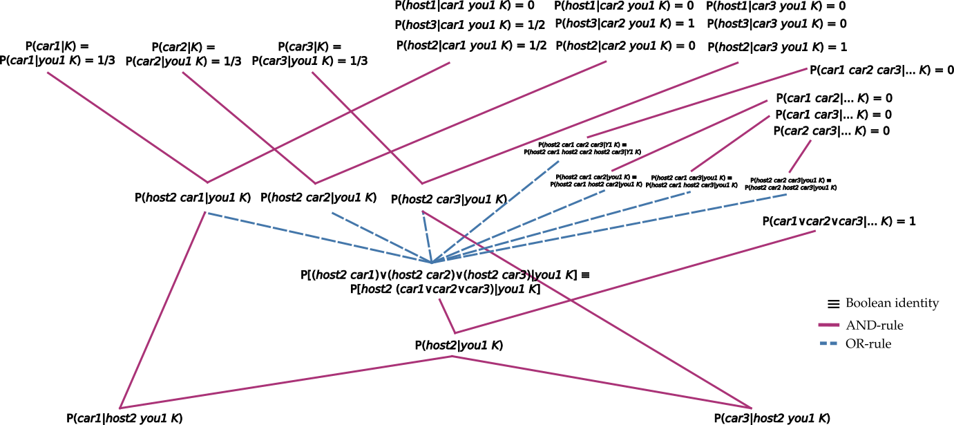
Note that we found these probabilities, and solved the Monty Hall problem, just by applying the fundamental rules of inference (§ 8.4), specifically the and-rule and or-rule, and the Boolean-algebra shortcut rules (§ 9), starting from given probabilities. Here is a depiction of how the fundamental and the shortcut rules connect the initial probabilities, at the top, to the final ones, at the bottom:

10.7 Remarks on the use of Bayes’s theorem

You notice that at several points our calculations could have taken a different path. For instance, in order to find \(\mathrm{P}(\mathsfit{\small car1} \nonscript\:\vert\nonscript\:\mathopen{} \mathsfit{\small host2} \mathbin{\mkern-0.5mu,\mkern-0.5mu}\mathsfit{\small you1} \mathbin{\mkern-0.5mu,\mkern-0.5mu}\mathsfit{K})\) we applied Bayes’s theorem to swap the sentences \(\mathsfit{\small car1}\) and \(\mathsfit{\small host2}\) in their proposal and conditional positions. Couldn’t we have swapped \(\mathsfit{\small car1}\) and \(\mathsfit{\small host2}\land \mathsfit{\small you1}\) instead? That is, couldn’t we have made a calculation starting with

\[ \mathrm{P}(\mathsfit{\small car1} \nonscript\:\vert\nonscript\:\mathopen{} \mathsfit{\small host2} \mathbin{\mkern-0.5mu,\mkern-0.5mu}\mathsfit{\small you1} \mathbin{\mkern-0.5mu,\mkern-0.5mu}\mathsfit{K}) =\frac{ \mathrm{P}(\mathsfit{\small host2} \mathbin{\mkern-0.5mu,\mkern-0.5mu}\mathsfit{\small you1}\nonscript\:\vert\nonscript\:\mathopen{} \mathsfit{\small car1} \mathbin{\mkern-0.5mu,\mkern-0.5mu}\mathsfit{K}) \cdot \mathrm{P}(\mathsfit{\small car1} \nonscript\:\vert\nonscript\:\mathopen{} \mathsfit{K}) }{\dotso} \enspace ? \]

after all, this is also a legitimate application of Bayes’s theorem.

The answer is: yes, we could have, and the final result would have been the same. The self-consistency of the probability calculus guarantees that there are no “wrong steps”, as long as every step is an application of one of the four fundamental rules (or of their shortcuts). The worst that can happen is that we take a longer route – but to exactly the same result. In fact it’s possible that there’s a shorter calculation route to arrive at the probabilities that we found in the previous section. But it doesn’t matter, because it would lead to the same result that we found.

10.8 Sensitivity analysis

In § 10.5 we briefly discussed possible interpretations or variations of the Monty Hall problem, for which the probability that the host chooses among the available doors 2 and 3 (if the car is behind the door you picked) is different from 50%.

When we want to know how an initial probability value can affect the final probabilities, we can leave its value as a variable, and check how the final probabilities change as we change this variable. This procedure is often called sensitivity analysis. Try to do a sensitivity analysis for the Monty Hall problem:

Exercise

Instead of assuming

\[\mathrm{P}(\mathsfit{\small host2} \nonscript\:\vert\nonscript\:\mathopen{} \mathsfit{\small car1} \mathbin{\mkern-0.5mu,\mkern-0.5mu}\mathsfit{\small you1} \mathbin{\mkern-0.5mu,\mkern-0.5mu}\mathsfit{K}) = \mathrm{P}(\mathsfit{\small host3} \nonscript\:\vert\nonscript\:\mathopen{} \mathsfit{\small car1} \mathbin{\mkern-0.5mu,\mkern-0.5mu}\mathsfit{\small you1} \mathbin{\mkern-0.5mu,\mkern-0.5mu}\mathsfit{K}) = 1/2\]

assign a generic variable value \(p\)

\[\mathrm{P}(\mathsfit{\small host2} \nonscript\:\vert\nonscript\:\mathopen{} \mathsfit{\small car1} \mathbin{\mkern-0.5mu,\mkern-0.5mu}\mathsfit{\small you1} \mathbin{\mkern-0.5mu,\mkern-0.5mu}\mathsfit{K}) = p \qquad \mathrm{P}(\mathsfit{\small host3} \nonscript\:\vert\nonscript\:\mathopen{} \mathsfit{\small car1} \mathbin{\mkern-0.5mu,\mkern-0.5mu}\mathsfit{\small you1} \mathbin{\mkern-0.5mu,\mkern-0.5mu}\mathsfit{K}) = 1-p\]

where \(p\) could be any value between \(0\) and \(1\).

Calculate \(\mathrm{P}(\mathsfit{\small car1} \nonscript\:\vert\nonscript\:\mathopen{} \mathsfit{\small host2} \mathbin{\mkern-0.5mu,\mkern-0.5mu}\mathsfit{\small you1} \mathbin{\mkern-0.5mu,\mkern-0.5mu}\mathsfit{K})\) as was done in the previous sections, but keeping \(p\) as a generic variable. This way you’ll find a probability \(\mathrm{P}(\mathsfit{\small car1} \nonscript\:\vert\nonscript\:\mathopen{} \mathsfit{\small host2} \mathbin{\mkern-0.5mu,\mkern-0.5mu}\mathsfit{\small you1} \mathbin{\mkern-0.5mu,\mkern-0.5mu}\mathsfit{K})\) that depends numerically on \(p\); it could be considered as a function of \(p\).
Plot how the value of \(\mathrm{P}(\mathsfit{\small car1} \nonscript\:\vert\nonscript\:\mathopen{} \mathsfit{\small host2} \mathbin{\mkern-0.5mu,\mkern-0.5mu}\mathsfit{\small you1} \mathbin{\mkern-0.5mu,\mkern-0.5mu}\mathsfit{K})\) depends on \(p\), as the latter ranges from \(0\) to \(1\).
For which range of values of \(p\) is it convenient to switch door, that is, \(\mathrm{P}(\mathsfit{\small car1} \nonscript\:\vert\nonscript\:\mathopen{} \mathsfit{\small host2} \mathbin{\mkern-0.5mu,\mkern-0.5mu}\mathsfit{\small you1} \mathbin{\mkern-0.5mu,\mkern-0.5mu}\mathsfit{K}) < 1/2\) ?
Imagine and describe alternative scenarios or background information that would lead to values of \(p\) different from \(0.5\).

10.9 Variations and further exercises

Exercise: other variations

In § 10.2 we decided that the agent in this inference was you, with the knowledge \(\mathsfit{K}\) right before you picked door 1. Try to change the agent: do you arrive at different probabilities?
- Consider a person in the audience, right before you picked door 1, as the agent, and re-solve the problem, adjusting all initial probabilities as needed.
- Consider the host as the agent, right before you picked door 1, and re-solve the problem, adjusting all initial probabilities as needed. Note that the host knows for certain where the car is, so you need to provide this additional, secret information. Consider the cases where the car is behind door 1 and behind door 3.

Suppose a friend of yours, backstage, gave you partial information about the location of the car (you cheater!), which makes you believe that the car should be closer to door 1. Assign the probabilities

\[\begin{aligned} \mathrm{P}(\mathsfit{\small car1} \nonscript\:\vert\nonscript\:\mathopen{} \mathsfit{K}') &= \mathrm{P}(\mathsfit{\small car1} \nonscript\:\vert\nonscript\:\mathopen{} \mathsfit{\small you1} \mathbin{\mkern-0.5mu,\mkern-0.5mu}\mathsfit{K}') = 1/3 + q \\ \mathrm{P}(\mathsfit{\small car2} \nonscript\:\vert\nonscript\:\mathopen{} \mathsfit{K}') &= \mathrm{P}(\mathsfit{\small car2} \nonscript\:\vert\nonscript\:\mathopen{} \mathsfit{\small you1} \mathbin{\mkern-0.5mu,\mkern-0.5mu}\mathsfit{K}') = 1/3 \\ \mathrm{P}(\mathsfit{\small car3} \nonscript\:\vert\nonscript\:\mathopen{} \mathsfit{K}') &= \mathrm{P}(\mathsfit{\small car3} \nonscript\:\vert\nonscript\:\mathopen{} \mathsfit{\small you1} \mathbin{\mkern-0.5mu,\mkern-0.5mu}\mathsfit{K}') = 1/3 - q \end{aligned} \]

with \(0 \le q \le 1/3\) (this background information is different from the previous one, so we denote it \(\mathsfit{K}'\)). Re-solve the problem keeping the variable \(q\), and find if there’s any value for \(q\) for which it’s best to keep door 1.

Exercise: making decisions

In this chapter we only solved the inference problem for the Monty Hall scenario. We calculated the probabilities of various outcomes. But no decision has been made yet.

Assign utilities to winning the car or winning the goat from the point of view of an agent who values the car more. The available decisions are, of course, “keep door 1” vs “switch to door 3”. Then solve the decision-making problem according to the procedure of § 37. What’s the optimal decision?
Now assign utilities from the point of view of an agent who values the goat more than the car. Then solve the decision-making problem according to the usual procedure. What’s the optimal decision?

Exercise: the Sleeping Beauty problem

Take a look at the inference problem presented in this video:

and try to solve it, not using intuition, but using the mechanical procedure and steps as in the Monty Hall solution above.

Note that the video asks “What do you believe is the probability that the coin came up heads?”. Since probability and degree of belief are the same thing, that is like asking “What do you believe is your belief that the coin came up heads?” which is a redundant or quirky question. Instead, simply answer the question “What is your degree of belief (that is, probability) that the coin came up heads?”.