36 Making decisions
\(\DeclarePairedDelimiter{\set}{\{}{\}}\) \(\DeclarePairedDelimiter{\abs}{\lvert}{\rvert}\)
36.1 Maximization of expected utility
In the previous chapter we associated utilities to consequences, that is, pairs \((\mathsfit{\color[RGB]{204,187,68}D}\mathbin{\mkern-0.5mu,\mkern-0.5mu}{\color[RGB]{238,102,119}Y\mathclose{}\mathord{\nonscript\mkern 0mu\textrm{\small=}\nonscript\mkern 0mu}\mathopen{}y})\) of decisions and outcomes. We can also associate utilities to the decisions alone – and these are used to determine the optimal decision.
The expected utility of a decision \(\mathsfit{\color[RGB]{204,187,68}D}\) in a basic decision problem is calculated as a weighted average over all possible outcomes, the weighs being the outcomes’ probabilities:
\[\mathrm{U}(\mathsfit{\color[RGB]{204,187,68}D}\nonscript\:\vert\nonscript\:\mathopen{}\mathsfit{I}) = \sum_{\color[RGB]{238,102,119}y} \mathrm{U}(\mathsfit{\color[RGB]{204,187,68}D}\mathbin{\mkern-0.5mu,\mkern-0.5mu}{\color[RGB]{238,102,119}Y\mathclose{}\mathord{\nonscript\mkern 0mu\textrm{\small=}\nonscript\mkern 0mu}\mathopen{}y} \nonscript\:\vert\nonscript\:\mathopen{} \mathsfit{I}) \cdot \mathrm{P}({\color[RGB]{238,102,119}Y\mathclose{}\mathord{\nonscript\mkern 0mu\textrm{\small=}\nonscript\mkern 0mu}\mathopen{}y} \nonscript\:\vert\nonscript\:\mathopen{} \mathsfit{\color[RGB]{204,187,68}D}\mathbin{\mkern-0.5mu,\mkern-0.5mu}{\color[RGB]{34,136,51}X\mathclose{}\mathord{\nonscript\mkern 0mu\textrm{\small=}\nonscript\mkern 0mu}\mathopen{}x} \mathbin{\mkern-0.5mu,\mkern-0.5mu}\mathsfit{\color[RGB]{34,136,51}data}\mathbin{\mkern-0.5mu,\mkern-0.5mu}\mathsfit{I}) \]
According to Decision Theory the agent’s final decision is determined by the
In the formula above, “\(\operatorname{argmax}\limits\limits_z G(z)\)” is the value \(z^*\) which maximizes the function \(G(z)\). Note the difference: \(\max\limits_z G(z)\) is the value of the maximum itself (its \(y\)-coordinate, so to speak), whereas \(\operatorname{argmax}\limits\limits_z G(z)\) is the value of the argument that gives the maximum (its \(x\)-coordinate). For instance
\[\max\limits_z (1-z)^2 = 0 \qquad\text{\small but}\qquad \operatorname{argmax}\limits\limits_z (1-z)^2 = 1\]
It may happen that there are several decisions which have equal, maximal expected utility. In this case any one of them can be chosen. A useful strategy is to choose one among them with equal probability. Such strategy helps minimizing the loss from possible small errors in the specification of the utilities, or from the presence of an antagonist agent which tries to predict what our agent is doing.
Numerical implementation in simple cases
The principle of maximal expected utility is straightforward to implement in many important problems.
In § 35.3 we represented the set of utilities by a utility matrix \(\boldsymbol{\color[RGB]{68,119,170}U}\). If the probabilities of the outcomes do not depend on the decisions, we represent them as a column matrix \(\boldsymbol{\color[RGB]{34,136,51}P}\), having one entry per outcome:
\[ \boldsymbol{\color[RGB]{34,136,51}P}\coloneqq \begin{bmatrix} \mathrm{P}({\color[RGB]{238,102,119}Y\mathclose{}\mathord{\nonscript\mkern 0mu\textrm{\small=}\nonscript\mkern 0mu}\mathopen{}y}' \nonscript\:\vert\nonscript\:\mathopen{} {\color[RGB]{34,136,51}X\mathclose{}\mathord{\nonscript\mkern 0mu\textrm{\small=}\nonscript\mkern 0mu}\mathopen{}x} \mathbin{\mkern-0.5mu,\mkern-0.5mu}\mathsfit{\color[RGB]{34,136,51}data}\mathbin{\mkern-0.5mu,\mkern-0.5mu}\mathsfit{I}) \\ \mathrm{P}({\color[RGB]{238,102,119}Y\mathclose{}\mathord{\nonscript\mkern 0mu\textrm{\small=}\nonscript\mkern 0mu}\mathopen{}y}'' \nonscript\:\vert\nonscript\:\mathopen{} {\color[RGB]{34,136,51}X\mathclose{}\mathord{\nonscript\mkern 0mu\textrm{\small=}\nonscript\mkern 0mu}\mathopen{}x} \mathbin{\mkern-0.5mu,\mkern-0.5mu}\mathsfit{\color[RGB]{34,136,51}data}\mathbin{\mkern-0.5mu,\mkern-0.5mu}\mathsfit{I}) \\ \dotso \end{bmatrix} \]
Then the collection of expected utilities is a column matrix, having one entry per decision, given by the matrix product \(\boldsymbol{\color[RGB]{68,119,170}U}\boldsymbol{\color[RGB]{34,136,51}P}\).
All that’s left is to check which of the entries in this final matrix is maximal.
36.2 Concrete example: targeted advertisement
As a concrete example application of the principle of maximal expected utility, let’s keep on using the adult-income task from chapter 33, in a typical present-day scenario.
Some corporation, which offers a particular phone app, wants to bombard its users with advertisements, because advertisement generates much more revenue than making the users pay for the app. For each user the corporation can choose one among three ad-types, let’s call them \({\color[RGB]{204,187,68}A}, {\color[RGB]{204,187,68}B}, {\color[RGB]{204,187,68}C}\). The revenue obtained from these ad-types depends on whether the target user’s income is \({\color[RGB]{238,102,119}{\small\verb;<=50K;}}\) or \({\color[RGB]{238,102,119}{\small\verb;>50K;}}\). A separate study run by the corporation has shown that the average revenues (per user per minute) depending on the three ad-types and the income levels are as follows:
| \(\mathit{\color[RGB]{238,102,119}income}\) | |||
| \({\color[RGB]{238,102,119}{\small\verb;<=50K;}}\) | \({\color[RGB]{238,102,119}{\small\verb;>50K;}}\) | ||
| ad-type | \({\color[RGB]{204,187,68}A}\) | \(\color[RGB]{68,119,170}-1\,\$\) | \(\color[RGB]{68,119,170}3\,\$\) |
| \({\color[RGB]{204,187,68}B}\) | \(\color[RGB]{68,119,170}2\,\$\) | \(\color[RGB]{68,119,170}2\,\$\) | |
| \({\color[RGB]{204,187,68}C}\) | \(\color[RGB]{68,119,170}3\,\$\) | \(\color[RGB]{68,119,170}-1\,\$\) | |
Ad-type \({\color[RGB]{204,187,68}B}\) is a neutral advertisement type that leads to revenue independently of the target user’s income. Ad-type \({\color[RGB]{204,187,68}A}\) targets high-income users, leading to higher revenue from them; but it leads to a loss if shown to the wrong target (more money spent on making and deploying the ad than what is gained from users’ purchases). Vice versa, ad-type \({\color[RGB]{204,187,68}B}\) targets low-income users, with a reverse effect.
The corporation doesn’t have access to its users’ income levels, but it covertly collects, through some other app, all or some of the eight predictor variates \(\color[RGB]{34,136,51}\mathit{workclass}\), \(\color[RGB]{34,136,51}\mathit{education}\), \(\color[RGB]{34,136,51}\dotsc\), \(\color[RGB]{34,136,51}\mathit{sex}\), \(\color[RGB]{34,136,51}\mathit{native\_country}\) from each of its users. The corporation has also access to the adult-income dataset (or let’s say a more recent version of it).
In this scenario the corporation would like to use an AI agent that can choose and show the optimal ad-type to each user.
Our prototype agent from chapters 31, 32, 33 can be used for such a task. It has already been trained with the dataset, and can use any subset (possibly even empty) of the eight predictors to calculate the probability for the two income levels.
All that’s left is to equip our prototype agent with a function that outputs the optimal decision, given the calculated probabilities and the set of utilities. In our code this is done by the function decide() described in chapter 32 and reprinted here:
-
decide(probs, utils=NULL) -
- Arguments:
-
probs: a probability distribution for one or more variates.utils: a named matrix or array of utilities. The rows of the matrix correspond to the available decisions, the columns or remaining array dimensions correspond to the possible values of the predictand variates.
- Output:
-
a list of elements
EUsandoptimal:EUsis a vector containing the expected utilities of all decisions, sorted from highest to lowest;optimalis the decision having maximal expected utility, or one of them, if more than one, selected with equal probability.
- Notes:
-
- If
utilsis missing orNULL, a matrix of the form \(\begin{bsmallmatrix}1&0&\dotso\\0&1&\dotso\\\dotso&\dotso&\dotso\end{bsmallmatrix}\) is assumed (which corresponds to using accuracy as evaluation metric).
- If
Example
A new user logs in; all eight predictors are available for this user:
\[\color[RGB]{34,136,51} \begin{aligned} &\mathit{workclass} \mathclose{}\mathord{\nonscript\mkern 0mu\textrm{\small=}\nonscript\mkern 0mu}\mathopen{}{\small\verb;Private;} && \mathit{education} \mathclose{}\mathord{\nonscript\mkern 0mu\textrm{\small=}\nonscript\mkern 0mu}\mathopen{}{\small\verb;Bachelors;} \\ & \mathit{marital\_status} \mathclose{}\mathord{\nonscript\mkern 0mu\textrm{\small=}\nonscript\mkern 0mu}\mathopen{}{\small\verb;Never-married;} && \mathit{occupation} \mathclose{}\mathord{\nonscript\mkern 0mu\textrm{\small=}\nonscript\mkern 0mu}\mathopen{}{\small\verb;Prof-specialty;} \\ & \mathit{relationship} \mathclose{}\mathord{\nonscript\mkern 0mu\textrm{\small=}\nonscript\mkern 0mu}\mathopen{}{\small\verb;Not-in-family;} && \mathit{race} \mathclose{}\mathord{\nonscript\mkern 0mu\textrm{\small=}\nonscript\mkern 0mu}\mathopen{}{\small\verb;White;} \\ & \mathit{sex} \mathclose{}\mathord{\nonscript\mkern 0mu\textrm{\small=}\nonscript\mkern 0mu}\mathopen{}{\small\verb;Female;} && \mathit{native\_country} \mathclose{}\mathord{\nonscript\mkern 0mu\textrm{\small=}\nonscript\mkern 0mu}\mathopen{}{\small\verb;United-States;} \end{aligned} \]
The agent calculates (using the infer() function) the probabilities for the two income levels, which turn out to be
\[ \begin{aligned} &\mathrm{P}({\color[RGB]{238,102,119}\mathit{\color[RGB]{238,102,119}income}\mathclose{}\mathord{\nonscript\mkern 0mu\textrm{\small=}\nonscript\mkern 0mu}\mathopen{}{\color[RGB]{238,102,119}{\small\verb;<=50K;}}} \nonscript\:\vert\nonscript\:\mathopen{} \mathsfit{\color[RGB]{34,136,51}predictor}, \mathsfit{\color[RGB]{34,136,51}data}, \mathsfit{I}) = 83.3\% \\&\mathrm{P}({\color[RGB]{238,102,119}\mathit{\color[RGB]{238,102,119}income}\mathclose{}\mathord{\nonscript\mkern 0mu\textrm{\small=}\nonscript\mkern 0mu}\mathopen{}{\color[RGB]{238,102,119}{\small\verb;>50K;}}} \nonscript\:\vert\nonscript\:\mathopen{} \mathsfit{\color[RGB]{34,136,51}predictor}, \mathsfit{\color[RGB]{34,136,51}data}, \mathsfit{I}) = 16.7\% \end{aligned} \]
and can be represented by the column matrix
\[\boldsymbol{\color[RGB]{34,136,51}P}\coloneqq \color[RGB]{34,136,51}\begin{bmatrix} 0.833\\0.167 \end{bmatrix} \]
The utilities previously given can be represented by the matrix
\[\boldsymbol{\color[RGB]{68,119,170}U}\coloneqq \color[RGB]{68,119,170}\begin{bmatrix} -1&3\\2&2\\3&-1 \end{bmatrix} \]
Multiplying the two matrices above we obtain the expected utilities of the three ad-types for the present user:
\[ \boldsymbol{\color[RGB]{68,119,170}U}\boldsymbol{\color[RGB]{34,136,51}P}= \color[RGB]{68,119,170}\begin{bmatrix} -1&3\\2&2\\3&-1 \end{bmatrix} \, \color[RGB]{34,136,51}\begin{bmatrix} 0.833\\0.167 \end{bmatrix}\color[RGB]{0,0,0} = \begin{bmatrix} {\color[RGB]{68,119,170}-1}\cdot{\color[RGB]{34,136,51}0.833} + {\color[RGB]{68,119,170}3}\cdot{\color[RGB]{34,136,51}0.167} \\ {\color[RGB]{68,119,170}2}\cdot{\color[RGB]{34,136,51}0.833} + {\color[RGB]{68,119,170}2}\cdot{\color[RGB]{34,136,51}0.167} \\ {\color[RGB]{68,119,170}3}\cdot{\color[RGB]{34,136,51}0.833} + ({\color[RGB]{68,119,170}-1})\cdot{\color[RGB]{34,136,51}0.167} \end{bmatrix} = \begin{bmatrix} -0.332\\ 2.000\\ \boldsymbol{2.332} \end{bmatrix} \]
The highest expected utility is that of ad-type \({\color[RGB]{204,187,68}C}\), which is therefore shown to the user.
Powerful flexibility of the optimal predictor machine
In the previous chapters we already emphasized and witnessed the flexibility of the optimal predictor machine with regard to the availability of the predictors: it can draw an inference even if some or all predictors are missing.
Now we can see another powerful kind of flexibility: the optimal predictor machine can in principle use different sets of decisions and different utilities for each new application. The decision criterion is not “hard-coded”; it can be customized on the fly.
The possible number of ad-types and the utilities could even be a function of the predictor values. For instance, there could be a set of three ad-types targeting users with \(\color[RGB]{34,136,51}\mathit{education}\mathclose{}\mathord{\nonscript\mkern 0mu\textrm{\small=}\nonscript\mkern 0mu}\mathopen{}{\small\verb;Bachelors;}\), a different set of four ad-types targeting users with \(\color[RGB]{34,136,51}\mathit{education}\mathclose{}\mathord{\nonscript\mkern 0mu\textrm{\small=}\nonscript\mkern 0mu}\mathopen{}{\small\verb;Preschool;}\), and so on.
36.3 “Unsystematic” decisions
In § 35.6 we emphasized the need to give appropriate utilities to outcomes, and to think about utilities in more general terms or with a more “open mind”, not simply equating them to monetary value, but considering all factors involved.
A similar open mind must be kept in determining the set of available decisions, considering the circumstances and also considering the decisions made by other agents. This leads to the idea of unsystematic decisions, more often called randomized decisions in the literature. Let’s illustrate the idea with an example.
Police Dispatch has received intel that a band of robbers is going to rob either location \(\mathsfit{\color[RGB]{204,187,68}A}\) or location \(\mathsfit{\color[RGB]{204,187,68}B}\). Dispatch can send a patrol to either of these places, but not both, owing to momentarily limited patrolling resources. The police patrol awaits orders from Dispatch on the radio.
Dispatch assigns a utility of, say, \(\color[RGB]{68,119,170}+1\) if the robbery is diverted and possibly the robbers caught, and a utility of \(\color[RGB]{68,119,170}0\) otherwise. As things stand, dispatching the patrol to either location has a 50% probability of catching the robbers, so each location decision has an expected utility of \(\color[RGB]{68,119,170}0.5\). But there’s a catch.
Dispatch has also received intel that the robbers are managing to intercept the radio transmission to the police patrol. So if Dispatch instructs the patrol to “go to location \(\mathsfit{\color[RGB]{204,187,68}A}\)”, the robbers will know that and rob location \(\mathsfit{\color[RGB]{204,187,68}B}\) instead. And vice versa if Dispatch sends the patrol to \(\mathsfit{\color[RGB]{204,187,68}B}\). The updated decision problem has now an expected utility of \(0\) for either choice.
What can Dispatch do? Well there’s at least one more possible decision. Dispatch can radio the patrol and instruct: “Toss a coin; if tails, go to \(\mathsfit{\color[RGB]{204,187,68}A}\); if heads, go to \(\mathsfit{\color[RGB]{204,187,68}B}\)”. If Dispatch does so, then the robbers, even intercepting the radio instruction, can’t to predict for certain where the police patrol will go. Should Dispatch make this third decision?
Draw the diagram for the basic decision problem above, with all three decisions, the outcomes of each, and the corresponding utilities and probabilities.
The third decision, “Toss a coin…” has an expected utility of \(0.5\), whereas the other two, “Go to \(\mathsfit{\color[RGB]{204,187,68}A}\)” or “Go to \(\mathsfit{\color[RGB]{204,187,68}B}\)”, have each \(0\) expected utility. The third decision is optimal among these three.
The crucial feature of the third decision is that it has an element of unpredictability for the robbers; it also has one for Dispatch, but that’s a side-effect.
This idea extends to more complex situations where an agent has an available sequence of decisions, the outcomes of each depending in turn on the decisions of another, antagonist agent. Such a sequence is usually called a strategy. The antagonist agent can in this case manipulate to some degree the outcomes, and alter its own strategy to minimize the first agent’s expected utilities and maximize its own. The first agent can remedy this by introducing a new set of decisions whose outcomes are instead unpredictable to the antagonist (and possibly to itself).
In a decision-making problem, several choices may happen to have equal, maximal expected utilities. In such situations it is usually recommended to “choose randomly” among those choices; this is what the function decide() (§ 36.2) does. This recommendation is an application of the ideas just discussed.
36.4 Multiple decisions: decision trees
Characteristics and graphical representation of a decision tree
In § 2.5 we discussed one important feature of Decision Theory: it can be applied in a sequential, recursive, or modular way. The typical case for such application is when further decisions are available if a specific outcome occurs. It would take several chapters to develop this more general application in full; here we summarize its main features and method.
Consider a set of decisions and outcomes, which depend on the occurrence of other outcomes and decisions, which in turn may depend on the occurrence of yet more outcomes and decisions, and so on. Graphically this situation can be represented by a decision tree, which depicts the sequences of decisions and outcomes in tree-like fashion. Here is an example:
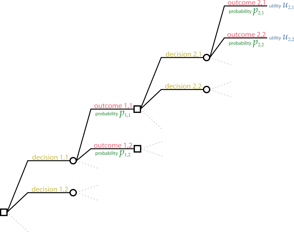
As usual, decision nodes are represented by squares, and inference nodes by circles. The root decision node is on the left. It presents a number of decisions which we can denote
\[\mathsfit{\color[RGB]{204,187,68}D}_{1,1},\quad \mathsfit{\color[RGB]{204,187,68}D}_{1,2},\quad\dotsc,\quad\mathsfit{\color[RGB]{204,187,68}D}_{1,\dotsc},\quad\dotsc\]
The first index “\({}_{1,}\)” indicates that these are root decisions; the second index enumerates these decisions. Each decision has a set of possible outcomes which we can denote, all together,
\[\mathsfit{\color[RGB]{34,136,51}O}_{1,1},\quad \mathsfit{\color[RGB]{34,136,51}O}_{1,2},\quad\dotsc,\quad\mathsfit{\color[RGB]{34,136,51}O}_{1,\dotsc},\quad\dotsc\]
with the same indexing convention. Each outcome has an associated degree of belief, which generally depends on the outcome and on the respective decision. For instance, the probability for outcome \(\mathsfit{\color[RGB]{34,136,51}O}_{1,1}\) must be written
\[\mathrm{P}(\mathsfit{\color[RGB]{34,136,51}O}_{1,1} \nonscript\:\vert\nonscript\:\mathopen{} \mathsfit{\color[RGB]{204,187,68}D}_{1,1} \mathbin{\mkern-0.5mu,\mkern-0.5mu}\mathsfit{I})\]
where \(\mathsfit{I}\) is the agent’s background information.
So far this looks almost like a basic decision tree (§ 3.1). Why “almost”? because we don’t associate utilities to these outcomes. Not yet. Instead, we see that some outcomes, like \(\mathsfit{\color[RGB]{34,136,51}O}_{1,1}\), open new decision nodes, with associated outcomes. We can keep the same notation convention as for the root decision node, but now using “\({}_{2,}\)” as first index:
\[\mathsfit{\color[RGB]{204,187,68}D}_{2,1},\quad \mathsfit{\color[RGB]{204,187,68}D}_{2,2},\quad\dotsc,\quad\mathsfit{\color[RGB]{204,187,68}D}_{2,\dotsc},\quad\dotsc\]
and for the their outcomes as well:
\[\mathsfit{\color[RGB]{34,136,51}O}_{2,1},\quad \mathsfit{\color[RGB]{34,136,51}O}_{2,2},\quad\dotsc,\quad\mathsfit{\color[RGB]{34,136,51}O}_{2,\dotsc},\quad\dotsc\]
Note that this is just a notation we use here; you can use any other convenient notation you like.
Each outcome of the second level has an associated degree of belief. Note that the degree of belief in an outcome generally depends on all previous decisions and outcomes leading to that outcome. For instance, the probability for outcome \(\mathsfit{\color[RGB]{34,136,51}O}_{2,2}\) must be written
\[\mathrm{P}(\mathsfit{\color[RGB]{34,136,51}O}_{2,2} \nonscript\:\vert\nonscript\:\mathopen{} \mathsfit{\color[RGB]{204,187,68}D}_{2,1} \mathbin{\mkern-0.5mu,\mkern-0.5mu}\mathsfit{\color[RGB]{34,136,51}O}_{1,1} \mathbin{\mkern-0.5mu,\mkern-0.5mu}\mathsfit{\color[RGB]{204,187,68}D}_{1,1} \mathbin{\mkern-0.5mu,\mkern-0.5mu}\mathsfit{I})\]
What about utilities? In this particular decision tree, the outcomes \(\mathsfit{\color[RGB]{34,136,51}O}_{2,1}\) and \(\mathsfit{\color[RGB]{34,136,51}O}_{2,2}\) do not lead to any subsequent possible decisions: they are among the tips of the tree. Then we do associate utilities to them: utilities are only associated to all outcomes at the tips of the decision tree. And it’s important to note that the utility associated to an outcome generally depends on all previous decisions and outcomes leading to that outcome. For instance, the utility associated to outcome \(\mathsfit{\color[RGB]{34,136,51}O}_{2,2}\) must be written
\[\mathrm{U}(\mathsfit{\color[RGB]{204,187,68}D}_{1,1} \mathbin{\mkern-0.5mu,\mkern-0.5mu}\mathsfit{\color[RGB]{34,136,51}O}_{1,1} \mathbin{\mkern-0.5mu,\mkern-0.5mu}\mathsfit{\color[RGB]{204,187,68}D}_{2,1} \mathbin{\mkern-0.5mu,\mkern-0.5mu}\mathsfit{\color[RGB]{34,136,51}O}_{2,2} \nonscript\:\vert\nonscript\:\mathopen{}\mathsfit{I})\]
Let’s summarize these important features of a general decision tree:
Decision making with a decision tree
Now to the important question: how do we choose the optimal decision at each decision node? The procedure, which is quite intuitive once one understands its general principle, is called averaging out and folding back or backwards induction. It starts from the tips, and step-wise associates a utility to each decision and each outcome, moving from the tips to the root of the decision tree:
A concrete example will be added
36.5 The full extent of Decision Theory
The simple decision-making problems and framework that we have discussed in these notes are only the basic blocks of Decision Theory. This theory covers more complicated decision problems. We only mention some examples:
- Sequential decisions. Many decision-making problems involve sequences of possible decisions, alternating with sequences of possible outcomes. These sequences can be represented as decision trees. Decision theory allows us to find the optimal decision sequence for instance through the “averaging out and folding back” procedure.
Uncertain utilities. It is possible to recast Decision Theory and the principle of maximal expected utility in terms, not of utility functions \(\mathrm{U}(\mathsfit{\color[RGB]{204,187,68}D}\mathbin{\mkern-0.5mu,\mkern-0.5mu}{\color[RGB]{238,102,119}Y\mathclose{}\mathord{\nonscript\mkern 0mu\textrm{\small=}\nonscript\mkern 0mu}\mathopen{}y} \nonscript\:\vert\nonscript\:\mathopen{} \mathsfit{I})\), but of probability distributions over utility values:
\[\mathrm{P}({\color[RGB]{68,119,170}U\mathclose{}\mathord{\nonscript\mkern 0mu\textrm{\small=}\nonscript\mkern 0mu}\mathopen{}u} \nonscript\:\vert\nonscript\:\mathopen{} \mathsfit{\color[RGB]{204,187,68}D}\mathbin{\mkern-0.5mu,\mkern-0.5mu}{\color[RGB]{238,102,119}Y\mathclose{}\mathord{\nonscript\mkern 0mu\textrm{\small=}\nonscript\mkern 0mu}\mathopen{}y} \mathbin{\mkern-0.5mu,\mkern-0.5mu}\mathsfit{I})\]
Formally the two approaches can be shown to be equivalent.
- Acquiring more information. In many situations the agent has one more possible choice: to gather more information in order to calculate sharper probabilities, rather than deciding immediately. This kind of decision is also accounted for by Decision Theory, and constitutes one of the theoretical bases of “reinforcement learning”.
- Multi-agent problems. To some extent it is possible to consider situations (such as games) with several agents having different and even opposing utilities. This area of Decision Theory is apparently still under development.