Working with R, I

Published

2025-09-16

As announced in the introduction, in these notes we use the R programming language to explore data science topics and for the software implementation of AI ideas.

R resources

There’s plenty of resources on installing R and learning its basics; you just have to do a short search and find the one that resonates with you. Examples:

There are also resources to run simple R scripts online:

R setup

There are various ways of working with R, as well as various Integrated Development Environments, which you can find with an online search. Use whatever you like best. In these notes we’ll write the code to run, which you can simply paste into an R console or run through your chosen software (note the copy icon on the right of each code snippet). It’s understood that you are using some working directory or folder, where you can load data and other files from, and where you save your results to.

Let’s start with something very simple. Here’s an input, and the output you should see:

2 + 1

[1] 3

Here’s another simple example (character strings in R are delimited by single quotes ' or double quotes "):

print('hello')

[1] "hello"

Let’s assign the value 5 to the variable x, then ask what x is; we also write a comment, introduced by one or more # signs:

## assign value to x
x <- 5

## output x
x

[1] 5

Now let’s assign the sequence of values \(0, -9, 4.7\) to x; this is done using the function c():

## assign values to x
x <- c(0, -9, 4.7)

## output x
x

[1]  0.0 -9.0  4.7

Let’s ask what is the second value in x; this is done with square brackets [ ]. Note that indexing starts from 1:

x[2]

[1] -9

We shall need some extra R packages to develop the material in these notes:

so let’s start an R session and install them.¹

¹ Depending on your operating system you can choose to install them as user, making them available only to you, or as superuser or administrator, making them available to every user in your machine.

install.packages('lpSolve')
install.packages('foreach')
install.packages('extraDistr')

We shall also use some custom-made functions for plotting and reading data. They are defined in the tplotfunctions.R file, which you should download to your working directory. Once it’s downloaded, you can load the functions this way:

source('tplotfunctions.R')

First exploration with R

As a very simple task to get acquainted with R, let’s do the following:

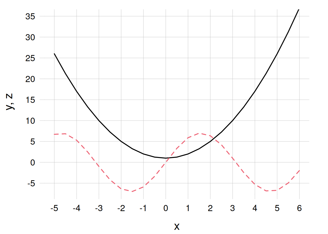
Assign the sequence of values form -5 to 5, in steps of 0.5, to the variable x.
Calculate \(x^2 + 1\) for each value contained in x, and assign the resulting values to the variable y.
Calculate \(7 \sin(x)\) for each value contained in x, and assign the resulting values to the variable z.
Plot the graphs of y vs x, and of z vs x, together, using different colours and line style, giving appropriate names to the axes, and choosing a range from -6 to 35 for the vertical axis.

We do all these operations, in sequence, below; note the comments:

x <- seq(from = -5, to = 6, by = 0.5)

y <- x^2 + 1

z <- 7 * sin(x)

tplot(
    x = x, y = y,
    col = 1, lty = 1,         ## colour and type of line
    ylim = c(-6, 35),         ## y-axis range
    xlab = 'x', ylab = 'y, z' ## axes labels
)

tplot(
    x = x, y = z,
    col = 2, lty = 2, ## different colour & type
    add = TRUE        ## add to previous plot
)

Looking at the code above you notice the following features:

Many functions, such as seq(), have named arguments, for example from = -5, or to = 6, or xlab = 'x'. In some cases the argument names can be omitted; for instance we could write seq(-5, 6, by = 0.5). But in these cases one must pay attention to the order of the arguments.
Most mathematical operations are performed element-wise on sequences of numbers.
In some circumstances it is possible to break a command over several lines; for instance, the arguments to the tplot() functions were not all given in one line. One must be careful because linebreaks do terminate some expressions; but in general it is safe – and clearer for people who read your code – to distribute function arguments across several lines, as done above.

Exercise 1

Get familiar with basic mathematical operations in R, like +, -, *, /, ^, exp(), log().
Get familiar to assigning single values and sequences of values to variables.
Check what happens when you change the colour and type of plot lines: try all numbers from 1 to 10.
Check what happens when you choose different ranges for the vertical axis in the first plot. Can you change the vertical range when you call the second plot?
What happens if you omit the vertical-axis range ylim = c(-6, 35)? (pay attention not to leave spurious commas.)
Check what happens if you specify a range for the horizontal axis with xlim =.