41 Neural networks
\(\DeclarePairedDelimiter{\set}{\{}{\}}\) \(\DeclarePairedDelimiter{\abs}{\lvert}{\rvert}\)
Neural networks are performing extremely well on complex tasks such as language modelling and realistic image generation, although the principle behind how they work, is quite simple.
The basic building block is a node, which receives some values as input, and computes a single output:
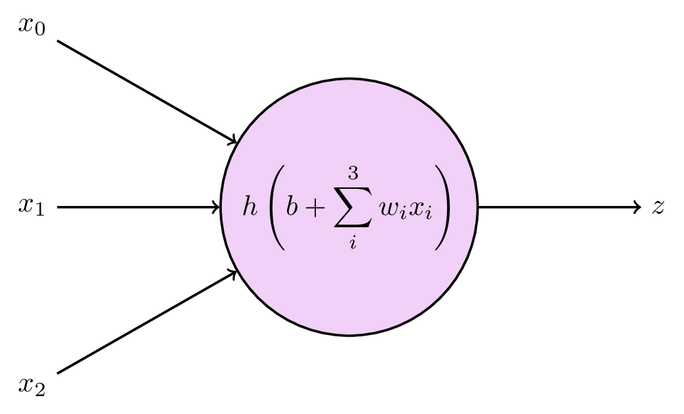
The output is computed from the inputs \(x_0, x_1, \dots, x_N\), each of which is multiplied by a weight \(w_1, w_2, \dots w_N\), and summed together along with an additional parameter \(b\), which is typically called a bias. You can probably identify this step as good old linear regression:
\[ a = b + \sum_{i=0}^N w_i x_i \,. \]
A key property to neural networks, however, is to introduce nonlinear relationships. This is done by evaluating the output from each node by an activation function \(h\). The final output \(z\) from the node is then
\[ z = h(a) = h \left( b + \sum_{i=0}^N w_i x_i \right) \]
The activation function is typically rather simple – the most popular is the rectified linear unit (ReLU), which propagates positive values but sets all negative values to zero:
\[ \text{ReLU}(x) = \max(0, x) \,. \]
Various other possibilities for choice of activation function exists, as we will explore in the exercises later.
Armed with our simple node, let us assemble several of them into a network. Starting with, say, four nodes, all the input data will be used by each of them: (todo) mention layers
Neural networks are great for several reasons. They can be arranged to work with practically any type of data, including unstructured data such as images or text, which is not neatly organised into a table of explicit feature values. Granted, this flexibility does not appear by (FIGURE) alone, but is due to clever additions to the network structure that is beyond the scope of our lectures. A more theoretical argument for neural networks comes from the universal approximation theorem, which states that
A neural network with a single hidden layer can be used to approximate any continuous function to any precision.
This is a very powerful property, which is explained in understandable terms here (the proof (CITE) is rather technical). But, as we know already, this only helps if we are trying to model something which has a functional relationship.
41.1 Training neural networks
Finding the optimal values of the model’s parameters \(\mathbf{w}\) is usually called to train the model. When we looked at polynomials in the machine learning introduction (Chapter 39) we did not talk about this yet, partly because polynomial models have a closed-form solution for the best parameters, meaning they can be computed directly. Since neural networks are nonlinear by design, analytic solutions are not available and we need a numerical approach; for instance: start with unsystematically chosen parameter values, then iteratively try to improve them.
Loss functions
The first step towards improving the parameters, is to define what improvement is. Ultimately, our goal is to make predictions about the data that equal the true values, which is to say, we want to minimise the difference between predictions \(f(\pmb{x}, \pmb{w}, \text{true values }y)\). This difference can be formulated in several different ways, but in the case of regression, the most common is the sum of squared errors:
\[ L(\mathbf{w}) = \sum_{\text{data points } i} (f(\mathbf{x}_i, \mathbf{w}) - y_i)^2 \]
\(L\) is called a loss function, alternatively a cost function or an error function. With this in place, the training process becomes a minimisation problem:
\[ \underset{\mathbf{w}}{\mathrm{arg\,min}}\, L(\mathbf{w}) \,. \tag{41.1}\]
To minimise the loss function we still need to apply it to some data \(\mathbf{x}\), but we have not made this dependence explicit, since the data are “unchanged” throughout the minimisation process.
As for any bounded function, the minimum can be found either where the gradient \(\nabla L(\mathbf{w})\) is zero, or where it does not exist. Solving this analytically is usually impossible, so we resort to a numerical solution – iteratively taking steps in the direction of smaller loss. The crucial point in neural network training is that the loss function is differentiable with respect to the network parameters, meaning we can compute \(\nabla L(\mathbf{w})\) and take steps in the negative (downwards) direction:
\[ \mathbf{w}^{n+1} = \mathbf{w}^{n} - \eta \nabla L(\mathbf{w}^{n}) \,. \tag{41.2}\]
This is the method of gradient descent. Here we have introduced a new hyperparameter \(\eta\) called the learning rate, which controls how large each step will be.
The process of actually adjusting the parameters in the correct direction is called backpropagation, and involves first computing the value of \(f(\mathbf{x}, \mathbf{w})\), and then stepping backwards through each layer of the network, recursively updating the parameters by using the derivative. This sounds very tedious, but can be done efficiently by automatic differentiation, i.e. letting a computer do it. Modern frameworks for neural network models require only to know the layout of the network, and will, as we shall see in the exercises, figure out the rest automatically.
Gradient descent
While we did not get into it earlier, the concept of defining a loss function and doing gradient descent, is in fact how the majority of machine learning algorithms are trained. Even for decision trees, which had their dedicated algorithm, we ended up with a loss minimisation task once we introduced boosting.
Straight-forward gradient descent as shown in equation {41.2} can work fine for relatively simple models, but will stop at the first minimum it encounters. For a reasonably complicated network, the loss function landscape can be expected to have several local minima or saddle points, causing the method to get stuck in places with suboptimal parameters. Several improved algorithms aim to tackle this.
- Stochastic gradient descent updates the parameters through equation {41.2} for only a subset of data at a time. This is more computationally efficient, and the stochastic element helps against getting stuck in a local minimum, since a local minimum for some subset of data might not be a minimum for a different subset.
- Adaptive gradient methods use different learning rates per parameter, which is updated for each iteration.
- Momentum methods remember the previous gradients and keeps moving in the same direction even through flat or uphill parts, like a massive rolling ball.
All of the above can be combined, and the most common method of doing so is the Adaptive Moment Estimation (Adam) algorithm.
42 Preventing overfitting - regularisation
In the previous chapter, we had several ways of limiting decision trees so they would not overfit to the training data. Many apply also here, but having introduced the concept of loss functions, we will add a general approach.
First, limiting complexity by tuning hyperparameters, is always an option. For a standard network, we can adjust the number of layers and the number of nodes per layer. Making good guesses about the architecture of the network is difficult, so a hyperparameter search is often necessary to develop a performant model.
Secondly, similar to random forests, one can make ensembles of models, trained on subsets (with replacement) of the data. For neural networks, however, this is less common, since the network is sort of an ensemble by itself. But remember that for random forests we also randomly dropped some of the features during training. The equivalent for neural networks is to randomly drop nodes, by zeroing their output for a single training iteration. This is called dropout.
Lastly, let us introduce general regularisation, which is based on modifying the loss function. This means it can be applied to any machine learning algorithm that minimises loss, and is not specific to the algorithm itself. What we want to do is to add a term in the loss function that penalises large parameter values. This way we do not need to restrict the explicit complexity of the model by changing the structure, but we rather restrict the “volume” the parameters can span out. The minimisation problem in equation {41.1} then becomes
\[ \underset{\mathbf{w}}{\mathrm{arg\,min}}\, L(\mathbf{w}) + \alpha ||\mathbf{w}||_p \,, \tag{42.1}\]
where the last part is the regularisation term, whose strength is controlled by a new hyperparameter, \(\alpha\). There are different ways of quantifying the values of the parameters \(\mathbf{w}\) – in the above equation we have written it generally as an \(p\)-norm, but to actually compute the value, we need to decide on which norm to use. The options are
- \(L^0\), or the zero norm: Defined as the number of parameters with non-zero values. Minimizing this would be similar to going into the model and removing parameters by hand. Unfortunately, as an optimisation task, this is extremely difficult and is just not a practical option.
- \(L^1\), which is the sum of the absolute values of the parameters: \(||\mathbf{w}||_1 = \sum_i |w_i|\). This is in statistics known as Lasso regularisation.
- \(L^2\), which is the Euclidean distance: \(||\mathbf{w}||_2 = \sum_i w_i^2\). This is also known as ridge regularisation, and is perhaps the most commonly used.
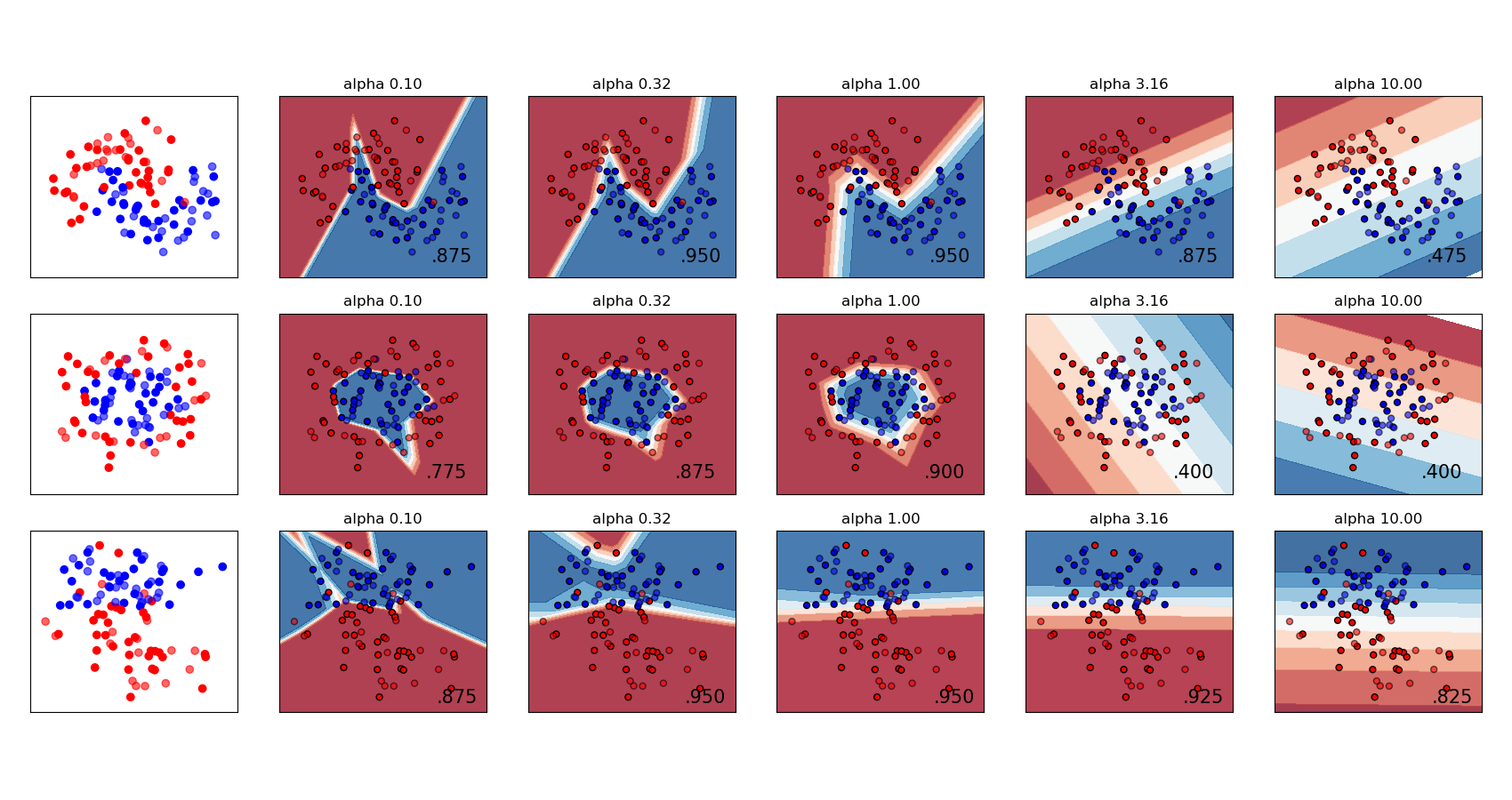
The scikit-learn User Guide has a nice example showing the effect of \(L^2\) regularisation for varying regularisation strength:
:
Regression: Follow the code examples in this notebook: neural_network_regression.ipynb
Classification: Follow the code examples in this notebook: neural_network_classification.ipynb
Real-world dataset classification: Make another attempt on the Adult Income dataset, this time using neural networks. Can you beat the tree-based models from last week? The training data are here:
https://github.com/pglpm/ADA511/raw/master/datasets/train-income_data_nominal_nomissing.csv, while the test data are here:https://github.com/pglpm/ADA511/raw/master/datasets/test-income_data_nominal_nomissing.csv