21 Statistics
\(\DeclarePairedDelimiter{\set}{\{}{\}}\) \(\DeclarePairedDelimiter{\abs}{\lvert}{\rvert}\)
21.1 What’s the difference between Probability Theory and Statistics?
“Probability theory” and “statistics” are often mentioned together. We shall soon see why, and what are the relationship between them. But first let’s try to define them more precisely:
- Probability theory
- is the theory that describes and norms the quantification and propagation of uncertainty, as we saw in § 8.1.
- Statistics
- is the study of collective properties of the variates of populations or, more generally, of collections of data.
There are clear and crucial differences between the two:
- The fact that we are uncertain about something doesn’t mean that there are populations or replicas involved. We can apply probability theory in situations that don’t involve any statistics.
- If we have full information about a population – the value of each variate for each unit – then we can calculate summaries and other properties of the variates. And there’s no uncertainty involved: at all times we can exactly calculate any information we like about any variates. So we do statistics, but probability theory plays no role.
Many texts do not clearly distinguish between probability and statistics. The distinction is important for us because we will have to solve problems involving the uncertainty about particular statistics, so the two must be kept clearly separate. This distinction was observed by James Clerk Maxwell who used it to develop the theories of statistical mechanics and kinetic theory.
In many concrete problems, however, probability theory and statistics do go hand in hand and interact. This happens mainly in two ways:
The statistics of a population give information that can be used in the conditional of an inference.
We want to draw inferences about some statistics of a population, whose values we don’t know.
Let’s now discuss some important statistics.
21.2 Frequencies and frequency distributions
Consider a statistical population of \(N\) units, with a variate \(X\) having a finite set of \(K\) values as domain. To keep things simple let’s just say these values are \(\set{1, 2, \dotsc, K}\) (without any ordering implied). Our discussion applies for any finite set. The variate \(X\) could be of any non-continuous type: nominal, ordinal, interval, binary (§ 12.2), or of a joint or complex type (§ 13). Let’s denote the variate associated with unit \(i\) by \(X_i\). For instance, we express that unit #3 has \(X\)-variate value \(5\) and unit #7 has \(X\)-variate value \(1\) by writing
\[ X_3 \mathclose{}\mathord{\nonscript\mkern 0mu\textrm{\small=}\nonscript\mkern 0mu}\mathopen{}5 \land X_7 \mathclose{}\mathord{\nonscript\mkern 0mu\textrm{\small=}\nonscript\mkern 0mu}\mathopen{}1 \quad\text{\small or equivalently}\quad X_3 \mathclose{}\mathord{\nonscript\mkern 0mu\textrm{\small=}\nonscript\mkern 0mu}\mathopen{}5 \mathbin{\mkern-0.5mu,\mkern-0.5mu}X_7 \mathclose{}\mathord{\nonscript\mkern 0mu\textrm{\small=}\nonscript\mkern 0mu}\mathopen{}1 \]
For each value \(a\) in the domain of the variate \(X\), we count how many units have that particular value. Let’s call the number we find \(n_a\). This is the absolute frequency of the value \(a\) in this population. Obviously \(n_a\) must be an integer between \(0\) (included) and \(K\) (included). The set of absolute frequencies of all values is called the absolute frequency distribution of the variate in the population. We must have
\[\sum_{a=1}^K n_a = N \ .\]
It is often useful to give the fraction of counts with respect to the population size, which we denote by \(f_a\):
\[f_a \coloneqq n_a/N\]
This is called the relative frequency of the value \(a\). Obviously \(0 \le f_a \le 1\). The collection of relative frequencies for all values, \(\set{f_1, f_2, \dotsc, f_K}\), satisfies
\[\sum_{a=1}^K f_a = 1 \ .\]
We call this collection of relative frequencies the relative frequency distribution. We shall denote it with the boldface symbol \(\boldsymbol{f}\) (boldface indicates that it is a tuple of numbers):
\(\boldsymbol{f} \coloneqq(f_1, f_2, \dotsc, f_K)\)
with an analogous convention if other letters are used instead of “\(f\)”.
The frequency distribution of values in a population does not give us full information about the population, because it doesn’t tell which unit has which value. In many situations, however, the frequencies are all we need to know, or all we can hope to know.
Frequencies and frequency distributions are quantities in the technical sense of § 12.1.1. In fact we can say, for instance, “The frequency of the value C is 0.3”, or “The frequency distribution for the values A, B, C is \((0.2, 0.7, 0.1)\)”. We shall denote the quantity, as separate from its value, by the corresponding capital letter, for example \(F_1\), so that we can write sentences about frequencies in our usual abbreviated form. For instance
\[ F_3\mathclose{}\mathord{\nonscript\mkern 0mu\textrm{\small=}\nonscript\mkern 0mu}\mathopen{}f_3 \]
means “The frequency of the variate value \(3\) is equal to \(f_3\)”, where \(f_3\) must be a specific number.
Consider the statistical population defined as follows:
- units: the bookings at a specific hotel during a specific time period
- variate: the market segment of the booking
- variate domain: the set of five values \(\set{{\small\verb;Aviation;}, {\small\verb;Complementary;}, {\small\verb;Corporate;}, {\small\verb;Offline;}, {\small\verb;Online;}}\)
The population data is stored in the file hotel_bookings-market.csv. Each row of the file corresponds to a unit, and lists the unit id (this is not a variate in the present population) and the market segment.
Use any method you like (a script in your favourite programming language, counting by hand, or whatever) to answer these questions:
- What is the size of the population?
- What are the absolute frequencies of the five values?
- What are their relative frequencies?
- Which units have the value \({\small\verb;Corporate;}\)?
Differences between frequencies and probabilities
The fact that frequencies are non-negative and sum up to 1 makes them somewhat similar to probabilities, from a purely numerical point of view. The two notions, however, are completely different and have different uses. Here is a list of some important differences:
Not few works in machine learning tend to call “probabilities” any set of positive numbers that sum up to one. Be careful when reading them. Mentally replace probability with degree of belief and see if the text mentioning “probabilities” still makes sense.
- A probability expresses a degree of belief.
- A frequency is the count of how many times something occurs.
- The probability of a sentence depends on an agent’s state of knowledge and background information. Two agents can assign different probabilities to the same sentence.
- The frequency of a value in a population is an objective physical quantity. All agents agree on the frequency (if they have the possibility of counting the occurrences).
- Probabilities refer to sentences.
- Frequencies refer to values in a population, not to sentences.
- A probability can refer to a specific unit in a population. An agent can consider, for instance, the probability that a variate for unit #7 has value
3. - A frequency cannot refer to a specific unit in a population. It is meaningless to “count how many times the value
3appears in unit #7”.
- A probability can refer to a specific unit in a population. An agent can consider, for instance, the probability that a variate for unit #7 has value
21.3 Joint frequencies
Consider the following population consisting of ten units with joint variate \((\mathit{age}, \mathit{race}, \mathit{sex}, \mathit{income})\), whose component variates have the following properties:
- \(\mathit{age}\): interval discrete with domain \(\set{17, 18, \dotsc, 90+}\)
- \(\mathit{race}\): nominal with domain \(\set{{\small\verb;Amer-Indian-Eskimo;}, {\small\verb;Asian-Pac-Islander;} , {\small\verb;Black;}, {\small\verb;Other;}, {\small\verb;White;}}\)
- \(\mathit{sex}\): binary with domain \(\set{{\small\verb;F;}, {\small\verb;M;}}\)
- \(\mathit{income}\): binary with domain \(\set{{\small\verb;`<=50K';}, {\small\verb;`>50K';}}\)
| \(\mathit{age}\) | \(\mathit{race}\) | \(\mathit{sex}\) | \(\mathit{income}\) |
|---|---|---|---|
| 53 | \({\small\verb;White;}\) | \({\small\verb;M;}\) | \({\small\verb;`>50K';}\) |
| 53 | \({\small\verb;Black;}\) | \({\small\verb;F;}\) | \({\small\verb;`<=50K';}\) |
| 48 | \({\small\verb;White;}\) | \({\small\verb;M;}\) | \({\small\verb;`>50K';}\) |
| 53 | \({\small\verb;White;}\) | \({\small\verb;F;}\) | \({\small\verb;`>50K';}\) |
| 53 | \({\small\verb;White;}\) | \({\small\verb;M;}\) | \({\small\verb;`<=50K';}\) |
| 26 | \({\small\verb;White;}\) | \({\small\verb;M;}\) | \({\small\verb;`<=50K';}\) |
| 48 | \({\small\verb;White;}\) | \({\small\verb;F;}\) | \({\small\verb;`>50K';}\) |
| 53 | \({\small\verb;White;}\) | \({\small\verb;M;}\) | \({\small\verb;`>50K';}\) |
| 53 | \({\small\verb;Black;}\) | \({\small\verb;M;}\) | \({\small\verb;`<=50K';}\) |
| 48 | \({\small\verb;Amer-Indian-Eskimo;}\) | \({\small\verb;M;}\) | \({\small\verb;`>50K';}\) |
The joint frequency distribution for the joint variate of the population above gives the frequencies of all possible joint variate values, for instance the value
\(\mathit{age}\mathclose{}\mathord{\nonscript\mkern 0mu\textrm{\small=}\nonscript\mkern 0mu}\mathopen{}53 \mathbin{\mkern-0.5mu,\mkern-0.5mu}\mathit{race}\mathclose{}\mathord{\nonscript\mkern 0mu\textrm{\small=}\nonscript\mkern 0mu}\mathopen{}{\small\verb;Black;}\mathbin{\mkern-0.5mu,\mkern-0.5mu}\mathit{sex}\mathclose{}\mathord{\nonscript\mkern 0mu\textrm{\small=}\nonscript\mkern 0mu}\mathopen{}{\small\verb;F;}\mathbin{\mkern-0.5mu,\mkern-0.5mu}\mathit{income}\mathclose{}\mathord{\nonscript\mkern 0mu\textrm{\small=}\nonscript\mkern 0mu}\mathopen{}{\small\verb;`<=50K';}\)
In this population, most joint values appear each only once, and the remaining values never appear; this is because of the population’s small size and the large number of possible variate values. A couple of joint values appear twice. We have for example
\[\begin{aligned} &f(\mathit{age}\mathclose{}\mathord{\nonscript\mkern 0mu\textrm{\small=}\nonscript\mkern 0mu}\mathopen{}53 \mathbin{\mkern-0.5mu,\mkern-0.5mu} \mathit{race}\mathclose{}\mathord{\nonscript\mkern 0mu\textrm{\small=}\nonscript\mkern 0mu}\mathopen{}{\small\verb;White;}\mathbin{\mkern-0.5mu,\mkern-0.5mu} \mathit{sex}\mathclose{}\mathord{\nonscript\mkern 0mu\textrm{\small=}\nonscript\mkern 0mu}\mathopen{}{\small\verb;M;}\mathbin{\mkern-0.5mu,\mkern-0.5mu} \mathit{income}\mathclose{}\mathord{\nonscript\mkern 0mu\textrm{\small=}\nonscript\mkern 0mu}\mathopen{}{\small\verb;`>50K';} ) = \frac{2}{10} \\[2ex] &f(\mathit{age}\mathclose{}\mathord{\nonscript\mkern 0mu\textrm{\small=}\nonscript\mkern 0mu}\mathopen{}53 \mathbin{\mkern-0.5mu,\mkern-0.5mu} \mathit{race}\mathclose{}\mathord{\nonscript\mkern 0mu\textrm{\small=}\nonscript\mkern 0mu}\mathopen{}{\small\verb;Black;}\mathbin{\mkern-0.5mu,\mkern-0.5mu} \mathit{sex}\mathclose{}\mathord{\nonscript\mkern 0mu\textrm{\small=}\nonscript\mkern 0mu}\mathopen{}{\small\verb;F;}\mathbin{\mkern-0.5mu,\mkern-0.5mu} \mathit{income}\mathclose{}\mathord{\nonscript\mkern 0mu\textrm{\small=}\nonscript\mkern 0mu}\mathopen{}{\small\verb;`<=50K';} ) = \frac{1}{10} \\[2ex] &f(\mathit{age}\mathclose{}\mathord{\nonscript\mkern 0mu\textrm{\small=}\nonscript\mkern 0mu}\mathopen{}48 \mathbin{\mkern-0.5mu,\mkern-0.5mu} \mathit{race}\mathclose{}\mathord{\nonscript\mkern 0mu\textrm{\small=}\nonscript\mkern 0mu}\mathopen{}{\small\verb;Amer-Indian-Eskimo;}\mathbin{\mkern-0.5mu,\mkern-0.5mu} \mathit{sex}\mathclose{}\mathord{\nonscript\mkern 0mu\textrm{\small=}\nonscript\mkern 0mu}\mathopen{}{\small\verb;F;}\mathbin{\mkern-0.5mu,\mkern-0.5mu} \mathit{income}\mathclose{}\mathord{\nonscript\mkern 0mu\textrm{\small=}\nonscript\mkern 0mu}\mathopen{}{\small\verb;`>50K';} ) = 0 \end{aligned}\]
Try to write a function that takes as input a dataset with a small number of variates and outputs the joint frequency distribution for all combinations of variate values. The best output format is a multidimensional array having one dimension per variate, and for each dimension a length equal to the number of possible values of that variate. The value of the array in each cell is the corresponding frequency.
For instance, consider the case of the income dataset above but without the age variate. The output of the function would then be an array with \(5 \times 2 \times 2\) dimensions
21.4 Marginal frequencies
When a population has a joint variate, we may be interested in only a subset of the simpler variates that constitute the joint one. In the population of the example above, for instance, we might be interested only in the \(\mathit{age}\) and \(\mathit{income}\) variates. These two variates together are then called marginal variates and define what we can call a marginal population of the original one. A marginal population has the same units as the original one, but only a subset of the variates of the original. It is a statistical population in its own right.
The notion of “marginalization” is a relative notion. Any population can often be considered as the marginal of a population with the same units but additional attributes.
Given a statistical population with joint variates \({\color[RGB]{34,136,51}X}, {\color[RGB]{238,102,119}Y}\), we define the marginal frequency of the value \({\color[RGB]{238,102,119}y}\) of \({\color[RGB]{238,102,119}Y}\) as the frequency of the value \({\color[RGB]{238,102,119}y}\) in the marginal population with the variate \({\color[RGB]{238,102,119}Y}\) alone. This frequency is simply written
\[ f({\color[RGB]{238,102,119}Y\mathclose{}\mathord{\nonscript\mkern 0mu\textrm{\small=}\nonscript\mkern 0mu}\mathopen{}y}) \]
A conditional frequency can be calculated as the sum of the joint frequencies for all values \({\color[RGB]{34,136,51}x}\), in a way analogous to marginal probabilities (§ 16.1):
\[ f({\color[RGB]{238,102,119}Y\mathclose{}\mathord{\nonscript\mkern 0mu\textrm{\small=}\nonscript\mkern 0mu}\mathopen{}y}) = \sum_{\color[RGB]{34,136,51}x} f({\color[RGB]{238,102,119}Y\mathclose{}\mathord{\nonscript\mkern 0mu\textrm{\small=}\nonscript\mkern 0mu}\mathopen{}y} \mathbin{\mkern-0.5mu,\mkern-0.5mu}{\color[RGB]{34,136,51}X\mathclose{}\mathord{\nonscript\mkern 0mu\textrm{\small=}\nonscript\mkern 0mu}\mathopen{}x}) \]
For example, if from the population of table 21.1 we consider the marginal population with variates \((\mathit{age}, \mathit{income})\), some of the marginal frequencies are
\[\begin{aligned} &f(\mathit{age}\mathclose{}\mathord{\nonscript\mkern 0mu\textrm{\small=}\nonscript\mkern 0mu}\mathopen{}53 \mathbin{\mkern-0.5mu,\mkern-0.5mu} \mathit{income}\mathclose{}\mathord{\nonscript\mkern 0mu\textrm{\small=}\nonscript\mkern 0mu}\mathopen{}{\small\verb;`<=50K';} ) = \frac{3}{10} \\[2ex] &f(\mathit{age}\mathclose{}\mathord{\nonscript\mkern 0mu\textrm{\small=}\nonscript\mkern 0mu}\mathopen{}26 \mathbin{\mkern-0.5mu,\mkern-0.5mu} \mathit{income}\mathclose{}\mathord{\nonscript\mkern 0mu\textrm{\small=}\nonscript\mkern 0mu}\mathopen{}{\small\verb;`<=50K';} ) = \frac{1}{10} \\[2ex] &f(\mathit{age}\mathclose{}\mathord{\nonscript\mkern 0mu\textrm{\small=}\nonscript\mkern 0mu}\mathopen{}48 \mathbin{\mkern-0.5mu,\mkern-0.5mu} \mathit{income}\mathclose{}\mathord{\nonscript\mkern 0mu\textrm{\small=}\nonscript\mkern 0mu}\mathopen{}{\small\verb;`>50K';} ) = \frac{3}{10} \end{aligned}\]
Download again the dataset
income_data_nominal_nomissing.csv:- Calculate the marginal frequencies of some of its variates.
- Does any variate have a value appearing with marginal absolute frequency equal to 1?
21.5 Summary statistics
In communicating statistics about a population it is always best to report and, when possible, visually show (for instance as marginal distributions) the full joint frequency distribution of the population’s variates.
Sometimes one wants to share some sort of “summary” of the frequency distribution, emphasizing particular aspects of it; because these are also aspects of the population. Different kinds of aspects can be chosen; some of them are only defined for specific types of variates. They are often called “summary statistics” or “descriptive statistics”. Below we give a brief description of some common ones, emphasizing when they are appropriate and when they are not. These summaries can also be used for probability distributions.
Mode
The mode is the value having the highest frequency (or probability, if we’re speaking about an agent’s beliefs rather than a population). There can be more than one mode.
The mode is defined for any distribution over discrete values, also for nominal quantities.
Median and quartiles
Recall (§ 12.2) that an ordinal or an interval quantity or variate have values that can be ranked in a specific order. If there is a value for which the sum of the frequencies of all values of rank lower than that value equals the sum of the frequencies of all values of rank higher than that value, then that value is called the median of the distribution. See the following histogram as an example:
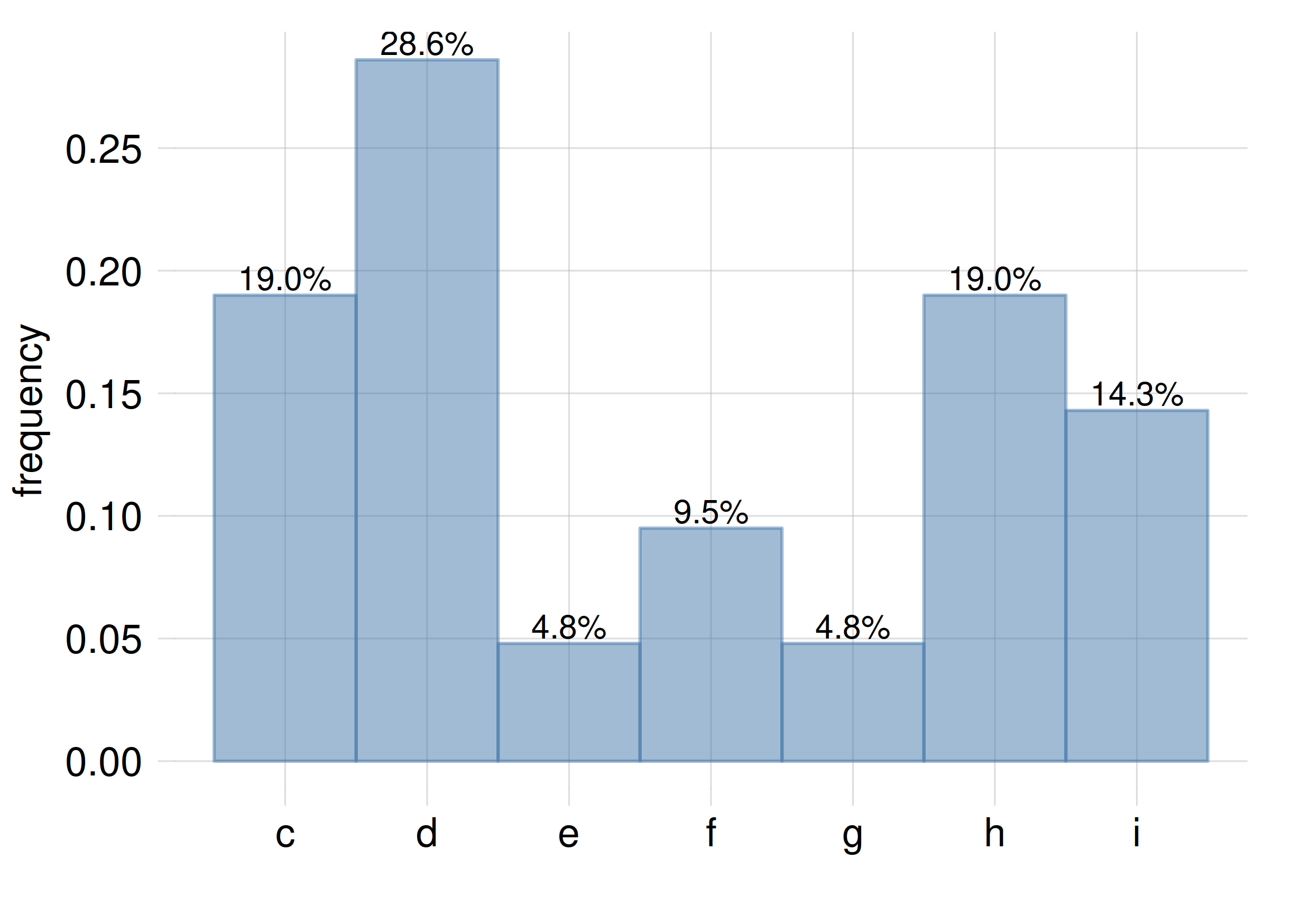 The value \({\small\verb;e;}\) is the median of this frequency distribution, because \(f({\small\verb;c;})+f({\small\verb;d;}) = f({\small\verb;f;})+f({\small\verb;g;})+f({\small\verb;h;})+f({\small\verb;i;})= 47.6\%\)
If there is no such separating value, then sightly different definitions of median exist in the literature; but the approximate idea is the same: a value that somehow divides the domain into two parts of roughly equal (50%) total frequency. This idea can be also applied to continuous distributions represented by densities.
The notion of median can be generalized to that of a value that separates the domain into a lower-rank part with total frequency 1/4, and a higher-rank part with total frequency 3/4; and also to that of a value separating into a 3/4 vs 1/4 proportion instead. These values are called the first quartile and third quartile. The two quartiles and the median (also called second quartile) divide the domain into four parts of roughly equal 25% frequencies.
If the variate or quantity under consideration is of interval type, then it’s possible to take the difference between the third and first quartile, called the interquartile range.
Mean and standard deviation
For an interval quantity \(X\) with values \(\set{x_1, x_2, \dotsc}\) for which it makes sense to take the sum, it is possible to define the mean and standard deviation:
\[ \bar{X} \coloneqq\sum_i x_i\cdot f(x_i) \qquad \sigma(X) \coloneqq\sqrt{\sum_i (x_i-\bar{X})^2\cdot f(x_i)} \]
we assume that their meaning is more or less familiar to you.
Uses and pitfalls
For a nominal variate or quantity it doesn’t make sense to speak of median, quartiles, mean, standard deviation, because its possible values cannot be ranked or added.
For an ordinal variate or quantity it doesn’t make sense to speak of mean or standard deviation, because its possible values cannot be added.
The mean and standard deviation can make sense and can be useful in some circumstances. But note that even if the values of a quantity can be summed, their mean (and standard deviation) may not quite make sense.
Consider the number of patients visiting a hospital in 100 consecutive days. It is possible to consider the mean number of patients per day. This number has a meaning: if this number of patients visited the hospital every day for 100 days, then the total number of visits would be equal to the actual total. The same reasoning can be made for the number of nurses working in the hospital every day for 100 days, and their mean.
Now consider the daily ratios of patients to nurses, for those 100 days. These ratios are numbers, so we can take their mean. But what does such a mean represent? if we multiply it by 100, we don’t obtain the total of anything. Also, if we consider the total number of patients and total number of nurses in 100 days, their ratio will not be equal to the “mean ratio” we calculated.
The example above is not meant to say that a mean of ratios never makes sense, but to point out that mean and standard deviation are often overused. In chapter 23 we will discuss other problems that may arise in using mean and standard deviation.
In general, when in doubt, we recommend to use median and quartiles or median and interquartile range, which are more generally meaningful and enjoy several other properties (for example so-called “robustness”) useful in doing statistics.
Note, in any case, that the present discussion regards the question of how to provide summary information besides the full frequency (or probability) distribution. If our problem is to choose one value out of the possible ones, then that’s a decision-making problem, which must be solved by specifying utilities and maximizing the expected utility, as preliminary discussed in chapter 2 and as will be discussed more in detail towards the final chapters.
21.6 Outliers vs out-of-population units
The term “outlier” frequently appears in problems related to statistics and probability, often in conjunction with some summary statistics described above. Unfortunately the definitions of this term can be confusing or misleading. With the notion of outlier often there also comes a barrage of “methods” or rules meant to “deal” with outliers. Some such rules, for instance the rule of discarding any datapoints lying at more than three standard deviations from the mean, are often mindless and dangerous.
So let’s avoid the term “outlier” for the moment, and let’s take a different perspective.
One reason why we consider a population of units is that we are interested in making inferences about some units in this population, for which we lack the values of some variates. As we shall see in the forthcoming chapters, such inferences can be made if we first try to infer the full joint frequency distribution for the variates of the population of interest.
This kind of inference becomes more difficult if we have reckoned into the population some units that actually don’t belong there.
Suppose for instance that a hospital is interested in the age of female patients admitted in a year. In collecting data, some male patients are counted in. Then obviously the age frequencies obtained from the collected data will not reflect the age frequencies among females. The problem is that some out-of-population units have been counted in by mistake.
The way out-of-population units affect and distort the frequency count can be different from problem to problem.
In our example, suppose that the wast majority of female patients could have age between 45–55 years, and that the male patients erroneously counted in also have age in the same range. Then the bulk of the frequency distribution will appear more inflated than it should be. Or suppose instead that the male patients erroneously reckoned have age between 80–90 years. In this case the old-age tail of the distribution will appear more inflated. As you see we can’t a priori point to any “tail” or “bulk” as a problem.
Low frequencies are relatively affected by out-of-population units more than high frequencies. Suppose 10 female patients out of 100 have age 52; frequency 10%. If one 52-year-old male patient is now included by mistake, the frequency becomes 11/101 ≈ 10.1%, or a 1% relative error. But if one female patient out of 100 has age 96 (1% frequency), and a male patient of the same age is now included by mistake, the frequency becomes 2/101 ≈ 1.98%, with a 98% relative error. This is the reason some people focus on distribution tails and “outliers”, defined as data having with low-frequency values. (Note that this reasoning would concern any regions of low frequency, for example among two modes; not just tails.)
Yet we cannot mindlessly attack low-frequency regions and data just because they could be more affected by out-of-population units. In many problems of data science, engineering, medicine, low-frequency cases are the most important ones (think of rare diseases, rare mineral elements, rare astronomical events, and so on). So if we alter or eliminate low-frequency data only because they might be out-of-population units, then we have dangerously affected all our inferences about such rare events.
Moreover, how could we judge what the “correct” frequency should be? Many outlier methods assume that the true frequency of the population has a Gaussian shape, and alter or cut the tails based on this assumption. But how can we know if such an assumption is correct? It turns out that the tails of a distribution are important for checking such assumption. Then you see the full circularity behind such mindless methods.
Which method should one use to face this problem, then? – The answer is that there’s no universal method. The approach depends on the specific problem. A data scientist must carefully examine all possible sources of out-of-population units, make inferences about them, and integrate these inferences in the general inference about the population of interest.
There is literature discussing first-principle approaches of this kind for different scenarios, but we cannot discuss them in the present course.